<?xml version="1.0" encoding="utf-8"?><feed xmlns="http://www.w3.org/2005/Atom" ><generator uri="https://jekyllrb.com/" version="4.3.4">Jekyll</generator><link href="https://blog.martisak.se/atom.xml" rel="self" type="application/atom+xml" /><link href="https://blog.martisak.se/" rel="alternate" type="text/html" /><updated>2024-10-03T20:20:02+00:00</updated><id>https://blog.martisak.se/atom.xml</id><title type="html">Martin’s blog</title><subtitle>Blogging about the life as a PhD student with focus on reproducible research.</subtitle><author><name>Martin Isaksson</name><email>martin@martisak.se</email></author><entry><title type="html">Our Research Recognized at 2023 IEEE Future Networks World Forum (FNWF)</title><link href="https://blog.martisak.se/2023/11/15/fnwf/" rel="alternate" type="text/html" title="Our Research Recognized at 2023 IEEE Future Networks World Forum (FNWF)" /><published>2023-11-15T00:00:00+00:00</published><updated>2023-11-15T00:00:00+00:00</updated><id>https://blog.martisak.se/2023/11/15/fnwf</id><content type="html" xml:base="https://blog.martisak.se/2023/11/15/fnwf/"><![CDATA[<p><strong>We are pleased to share some news from the  2023 IEEE Future Networks World Forum (FNWF) in Baltimore, MD, USA. Our paper, <a href="/publications/mmwave-beam-selection-in-analog-beamforming-using-personalized-federated-learning/">mmWave Beam Selection in Analog Beamforming Using Personalized Federated Learning</a> was awarded the Best Paper Award. This recognition is both humbling and encouraging for us as researchers.</strong></p>

<!-- more -->

<div class="container figure">
<div class="row">
    <div class="col-md-12">
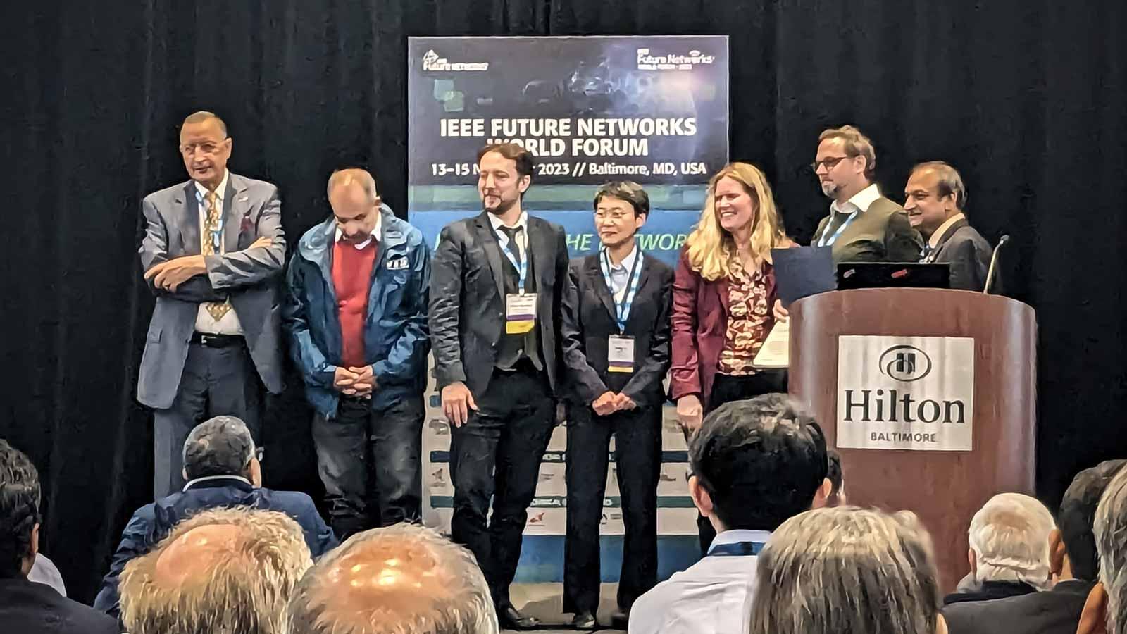
        <div><img src="/assets/images/fnwf1.jpg" alt="Best Paper Award ceremony at the IEEE FNWF banquet." /></div>
        <div class="caption">Best Paper Award ceremony at the IEEE FNWF banquet. Photo by Thomas Sandholm.</div>
    </div>
</div>
</div>

<p>This achievement is not ours alone. It reflects the support and collaboration of many - from our colleagues and mentors to the broader community of researchers and professionals who continually inspire us. Our sincere thanks go to the <a href="https://fnwf2023.ieee.org/">IEEE FNWF</a> for considering our work and to everyone involved in the conference.</p>

<p>A special mention to my co-authors Filippo Vannella, David Sandberg, and Rickard Cöster. Your insights and hard work were crucial in this endeavor. Working with you has been a rewarding experience. Toghether, we also extend our gratitude to all who contributed in various capacities, not least the coffee roasters who kept us going!</p>

<p>Congratulations to the other awardees. It’s an honor to be recognized alongside such talented peers.</p>

<p>For those interested, our paper is available <a href="/publications/mmwave-beam-selection-in-analog-beamforming-using-personalized-federated-learning/">here</a>. We welcome your thoughts and engagement. Lastly, a thank you to Thomas Sandholm for capturing the pinnacle of our journey in this photograph.</p>

<p>We look forward to continuing our research and sharing our findings with the community.</p>

<div class="container figure">
<div class="row">
    <div class="col-md-12">
        <div><img src="/assets/images/fnwf2.jpg" alt="Best Paper Award at the IEEE FNWF 2023." /></div>
        <div class="caption">Our paper, <a href="/publications/mmwave-beam-selection-in-analog-beamforming-using-personalized-federated-learning/">mmWave Beam Selection in Analog Beamforming Using Personalized Federated Learning</a> was awarded the Best Paper Award.</div>
    </div>
</div>
</div>]]></content><author><name>Martin Isaksson</name><email>martin@martisak.se</email></author><category term="Publications" /><category term="academia" /><category term="latex" /><category term="link" /><summary type="html"><![CDATA[We are pleased to share some news from the 2023 IEEE Future Networks World Forum (FNWF) in Baltimore, MD, USA. Our paper, mmWave Beam Selection in Analog Beamforming Using Personalized Federated Learning was awarded the Best Paper Award. This recognition is both humbling and encouraging for us as researchers.]]></summary><media:thumbnail xmlns:media="http://search.yahoo.com/mrss/" url="https://blog.martisak.se/images/blog-ai.jpg" /><media:content medium="image" url="https://blog.martisak.se/images/blog-ai.jpg" xmlns:media="http://search.yahoo.com/mrss/" /></entry><entry><title type="html">Optimizing Your LaTeX Workflow: A Guide to Choosing a Build System</title><link href="https://blog.martisak.se/2023/10/01/compiling/" rel="alternate" type="text/html" title="Optimizing Your LaTeX Workflow: A Guide to Choosing a Build System" /><published>2023-10-01T00:00:00+00:00</published><updated>2023-10-01T00:00:00+00:00</updated><id>https://blog.martisak.se/2023/10/01/compiling</id><content type="html" xml:base="https://blog.martisak.se/2023/10/01/compiling/"><![CDATA[<p><strong>Long LaTeX build times can be a significant challenge for researchers and
developers, hampering productivity and efficiency. This issue arises due to the
complexity of LaTeX documents and the diversity of build systems available. We
present a comprehensive exploration of LaTeX build systems, helping authors
choose the most suitable one. By identifying the best build system, authors can
streamline their workflow, reduce build times, and ultimately enhance their
research and development endeavors.</strong></p>

<!-- more -->

<h2 id="introduction">Introduction</h2>

<p>I still remember the issues I had, many years ago, trying to build <a href="/publications/anisotropic">my Master
thesis report</a> using <code class="language-plaintext highlighter-rouge">latex</code> and <code class="language-plaintext highlighter-rouge">dvips</code>. Since then
my build process has gone through a few iterations, to simplify, to make it
faster, or to accommodate some new thing that I learned. Frustrated by the long
build times, I have tried many things which may or may not have helped. The
discussion (for example  <i class="ai ai-stackoverflow-square"></i> <a href="https://tex.stackexchange.com/questions/8791/speeding-up-latex-compilation">Speeding up LaTeX
compilation</a>)
seems to be plagued by hearsay. For a typesetting system that is used by
scientists, the discussion is unexpectedly remarkably unscientific.</p>

<p>In this blog post we will embark on an exploration of this rabbit hole,
unraveling the intricacies of different LaTeX build systems. We will dive deep
into the world of LaTeX compilation methods, comparing and contrasting different
local build methods. By the end, you’ll be equipped with the knowledge to choose
the right path for your next LaTeX adventure.</p>

<!-- https://tex.stackexchange.com/questions/6374/what-are-the-pros-and-cons-pertaining-to-latex-dvipdfm-versus-latex-dvi
https://tex.stackexchange.com/questions/18987/how-to-make-the-pdfs-produced-by-pdflatex-smaller -->

<h2 id="background">Background</h2>

<h3 id="why-dont-just-use-overleaf">Why don’t just use Overleaf?</h3>

<p><i class="ai ai-overleaf-square"></i> <a href="https://www.overleaf.com/">Overleaf</a> is fantastic, but a local LaTeX build environment can offer advantages over Overleaf in certain situations. A key benefit is control. With a local setup, users have complete control over their LaTeX distribution, packages, configuration and development environment. For me, the enhanced privacy and security is the most important reason to using a local build environment.</p>

<p>It is important to note that <i class="ai ai-overleaf-square"></i> <a href="https://www.overleaf.com/">Overleaf</a> excels in collaborative and cloud-based scenarios when teams working on LaTeX documents can work simultaneously in the same document. <i class="ai ai-overleaf-square"></i> <a href="https://www.overleaf.com/">Overleaf</a> allows real-time collaboration with version control and seamless sharing and also eliminates the need to install and manage LaTeX distributions and packages, making it accessible to users who may not be experienced installing complex software such as LaTeX.</p>

<h3 id="installing-latex">Installing LaTeX</h3>

<p>Your method of installing LaTeX varies with your operating system, the level of control you want, and other constraints. We will not go into this in detail here, see <a href="https://www.latex-project.org/get/">Getting LaTeX</a> and <a href="https://www.tug.org/interest.html#free">Free TeX implementations</a>.</p>

<h3 id="building-a-latex-document">Building a LaTeX document</h3>

<p>LaTeX employs a multi-pass typesetting process to enable various features like table of contents, lists of figures, cross-referencing, glossaries, indexing, and bibliographic citations. In this process, the data generated during one pass (compilation) is saved to intermediate files and then serves as input for any subsequent passes.</p>

<script src="/assets/js/mermaid.min.js"></script>
<div class="mermaid">
graph LR;
    .tex--&gt;|latex|.dvi;
    .tex--&gt;|pdflatex, xelatex|.pdf;
    .dvi--&gt;|dvips|.ps;
    .ps--&gt;|ps2pdf|.pdf;
    .dvi--&gt;|dvipdfm, dvipdfmx|.pdf;
</div>

<p>We have many choices to make here (see <i class="ai ai-stackoverflow-square"></i> <a href="https://tex.stackexchange.com/questions/6374/what-are-the-pros-and-cons-pertaining-to-latex-dvipdfm-versus-latex-dvi">What are the pros and cons pertaining to
“latex -&gt; dvipdfm” versus “latex -&gt; dvips -&gt;
ps2pdf”?</a>
), but in this case we know we want a Portable Document Format (PDF), <code class="language-plaintext highlighter-rouge">.pdf</code>,
file. There are some differences depending on which workflow we pick here, but
for this document we can pick any of them.</p>

<p>The multi-pass typesetting process involves several steps to create a PDF
document with references using BibTeX and glossaries using <code class="language-plaintext highlighter-rouge">makeglossaries</code>:</p>

<ol>
  <li>
    <p><strong>Compilation with LaTeX</strong>. First we run <code class="language-plaintext highlighter-rouge">pdflatex</code> on the input <code class="language-plaintext highlighter-rouge">.tex</code> file.
This initial compilation generates an intermediate <code class="language-plaintext highlighter-rouge">.aux</code> file containing
information about citations, cross-references, and glossary entries. Since we
are using the package <code class="language-plaintext highlighter-rouge">glossaries-extra</code>, we also get a <code class="language-plaintext highlighter-rouge">makeindex</code> style
file <code class="language-plaintext highlighter-rouge">.ist</code> and an <code class="language-plaintext highlighter-rouge">.acn</code> file.</p>
  </li>
  <li>
    <p><strong>BibTeX for References</strong> If we have references in our document, we need to
run BibTeX on the <code class="language-plaintext highlighter-rouge">.aux</code> file. BibTeX reads our bibliography database
(<code class="language-plaintext highlighter-rouge">.bib</code>) and generates a <code class="language-plaintext highlighter-rouge">.bbl</code> file, which contains the formatted reference
information.</p>
  </li>
  <li>
    <p><strong>Glossaries with <code class="language-plaintext highlighter-rouge">makeglossaries</code></strong> If we have a glossary in our document,
we use <code class="language-plaintext highlighter-rouge">makeglossaries</code> on the <code class="language-plaintext highlighter-rouge">.aux</code> file. <code class="language-plaintext highlighter-rouge">makeglossaries</code> reads the
glossary definitions and generates the necessary files to include glossary
entries in our document.</p>
  </li>
  <li>
    <p><strong>LaTeX Compilation (2nd Pass)</strong> Now we need to run <code class="language-plaintext highlighter-rouge">pdflatex</code> on the <code class="language-plaintext highlighter-rouge">.tex</code>
file again. This time, LaTeX incorporates the formatted references from the
<code class="language-plaintext highlighter-rouge">.bbl</code> file into our document. If there are any citations, they will be
correctly numbered and formatted in the reference list, but the citations
themselves will be rendered as <code class="language-plaintext highlighter-rouge">[?]</code>.</p>
  </li>
  <li>
    <p><strong>LaTeX Compilation (3rd Pass)</strong> Running <code class="language-plaintext highlighter-rouge">pdflatex</code> on the <code class="language-plaintext highlighter-rouge">.tex</code> file once
more ensures that glossary entries are properly integrated into your document
and that citations are properly numbered.</p>
  </li>
  <li>
    <p><strong>Final compilations</strong> We need to repeat the <code class="language-plaintext highlighter-rouge">pdflatex</code> compilation step as
many times as needed to resolve all cross-references and ensure the document
is correctly formatted. LaTeX may issue warnings or errors during this
process that need to be addressed. In our case, for this document, we only
need to run <code class="language-plaintext highlighter-rouge">pdflatex</code> three times in total.</p>
  </li>
  <li>
    <p><strong>PDF Generation</strong> Once all the necessary information is integrated into your
document, a PDF file is generated as the output.</p>
  </li>
</ol>

<div class="container">
    <div class="row">
        <div class="col-md-12">
            <iframe width="560" height="315" src="https://www.youtube.com/embed/iqk5uJPo6_E?si=B8U5kkCp76DxrHk5" title="YouTube video player" frameborder="0" allow="accelerometer; autoplay; clipboard-write; encrypted-media; gyroscope; picture-in-picture; web-share" allowfullscreen=""></iframe>
        </div>
    </div>
</div>

<p>See <i class="ai ai-stackoverflow-square"></i> <a href="https://tex.stackexchange.com/questions/7770/file-extensions-related-to-latex-etc">File extensions related to LaTeX, etc</a> and <i class="fa-brands fa-square-github"></i> <a href="https://github.com/wspr/latex-auxfiles">latex-auxfiles</a> for more information on different file formats that you might encounter during the build process.</p>

<h2 id="method">Method</h2>

<h3 id="the-document">The document</h3>

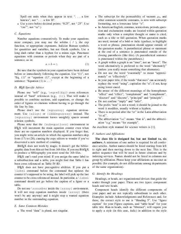
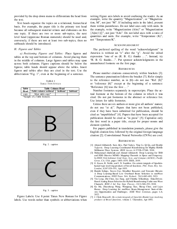
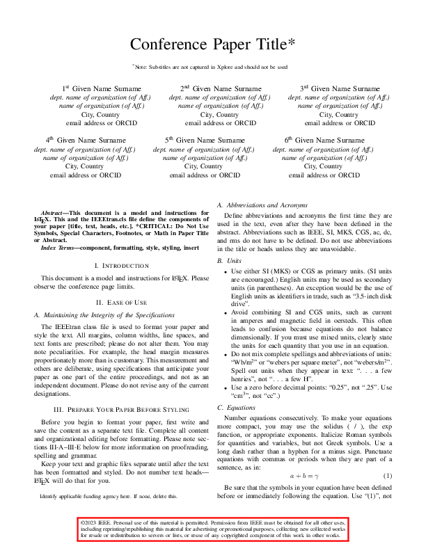
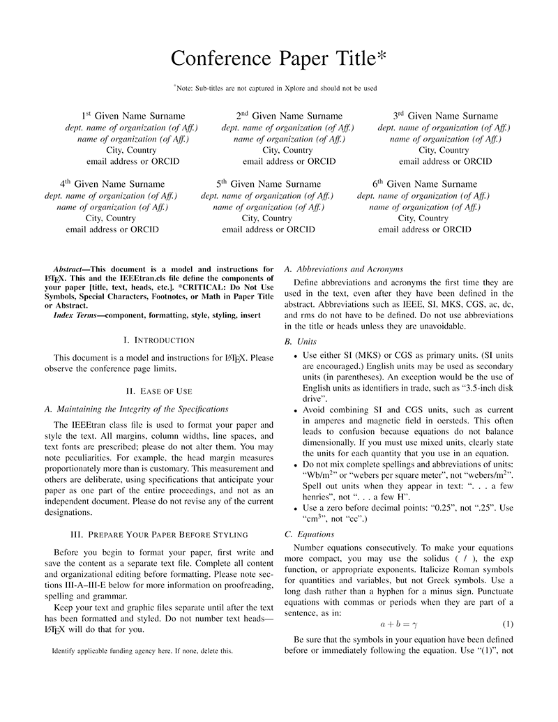
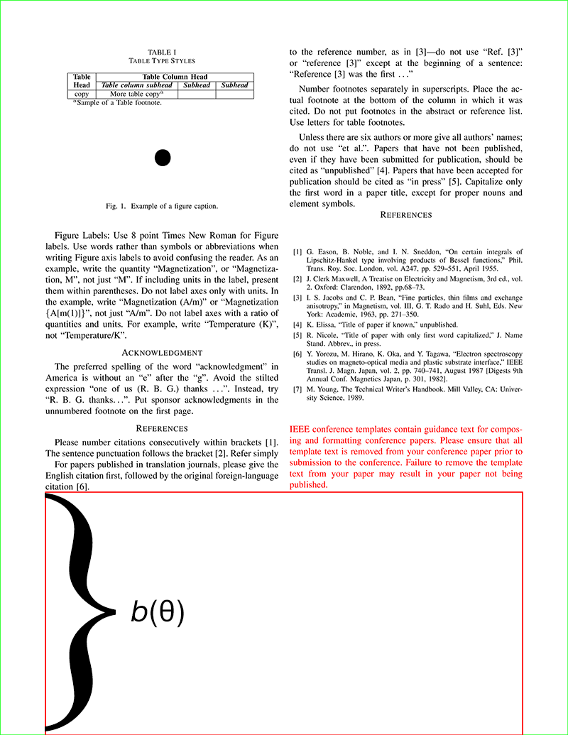
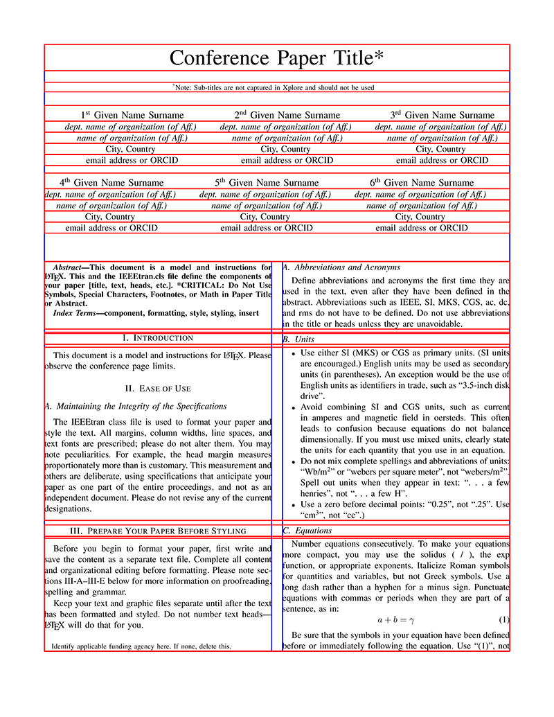
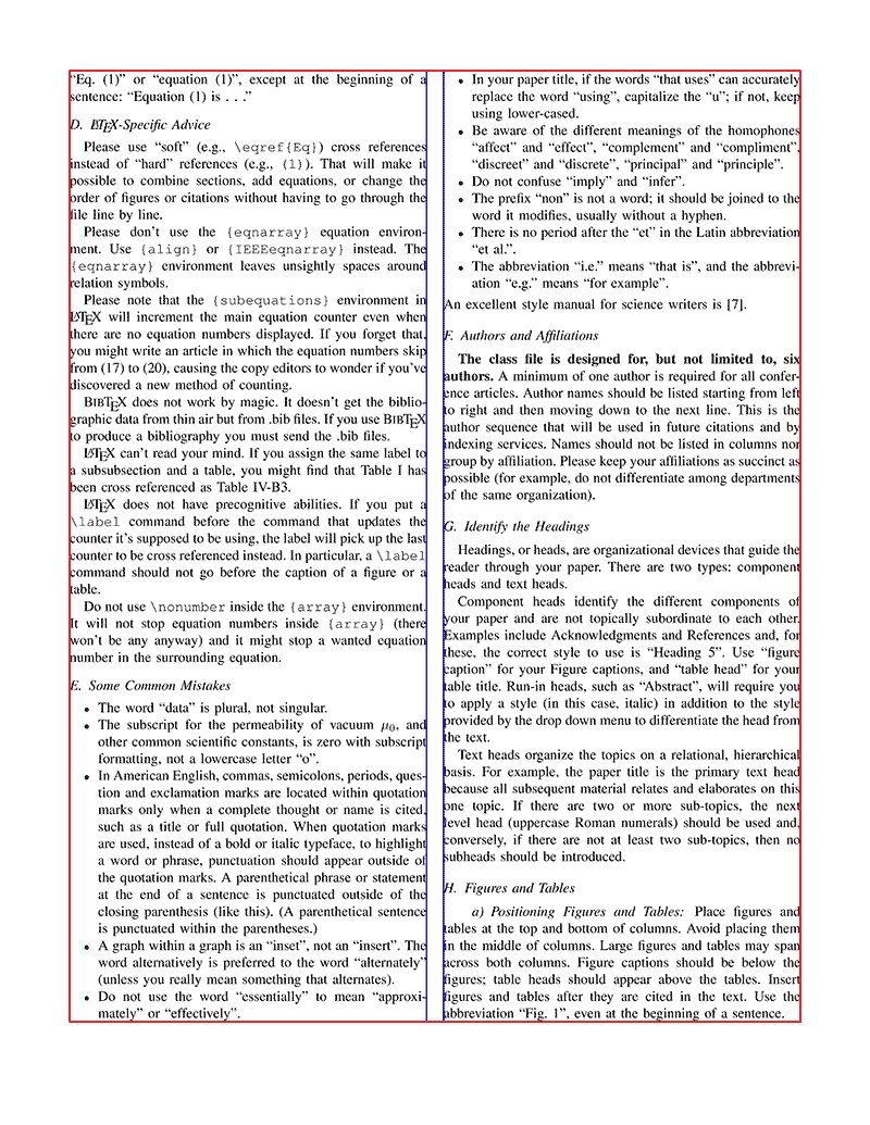
<p>The example document we will use in the remainder of this post is based on the
<i class="ai ai-ieee"></i> <a href="https://www.ieee.org/conferences/publishing/templates.html">IEEE conference
template</a> <a class="citation" href="#shell2002use">(Shell, 2002)</a>. We will make some changes, for example adding a reference file
using BiBTeX and a glossary using the <code class="language-plaintext highlighter-rouge">glossaries-extra</code> package. We will also
add three example figures. These figures are available both in <code class="language-plaintext highlighter-rouge">.eps</code> and <code class="language-plaintext highlighter-rouge">.pdf</code>
format, so that we don’t need to run an expensive conversion process for each
figure. We will include these figures without the file suffix, for example</p>

<figure class="highlight"><pre><code class="language-tex" data-lang="tex"><table class="rouge-table"><tbody><tr><td class="gutter gl"><pre class="lineno">1
</pre></td><td class="code"><pre><span class="k">\includegraphics</span><span class="na">[width=.9\linewidth]</span><span class="p">{</span>example-image-a<span class="p">}</span>.
</pre></td></tr></tbody></table></code></pre></figure>

<div class="container figure">
<div class="row">
    <div class="col-md-6">
        <div><img src="/assets/images/test-paper-0.png" alt="" class="border" /></div>
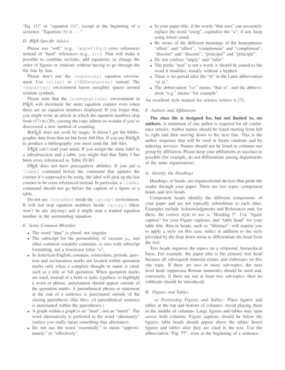
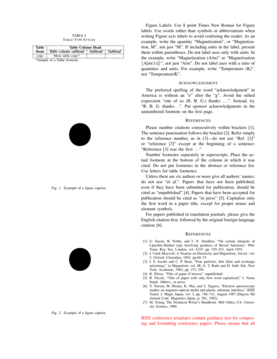
        <div class="caption">The <b>first page</b> contains our title and a figure.</div>
    </div>
    <div class="col-md-6">
        <div><img src="/assets/images/test-paper-1.png" alt="" class="border" /></div>
        <div class="caption">The <b>second page</b> contains some references.</div>
    </div>
</div>
<div class="row">
    <div class="col-md-6">
        <div><img src="/assets/images/test-paper-2.png" alt="" class="border" /></div>
        <div class="caption">The <b>third page</b> contains the reference list and an acronym.</div>
    </div>
    <div class="col-md-6">
        <div><img src="/assets/images/test-paper-3.png" alt="" class="border" /></div>
        <div class="caption">The last and <b>fourth page</b> contains the list of acronyms.</div>
    </div>
</div>
</div>

<p>There are many things that effect the compilation times of a LaTeX document. See
<i class="ai ai-stackoverflow-square"></i> <a href="https://tex.stackexchange.com/questions/197745/what-affects-compilation-times-especially-in-longer-documents">What affects compilation times,
especially in longer
documents?</a>.
The document we use here is short and doesn’t contain a lot of features, and we
do this to keep compilation times low since we will be repeating this build many
times.</p>

<p>You can view the <i class="ai ai-overleaf-square"></i> <a href="https://www.overleaf.com/read/hytfmxnyymnf">source code for this document on Overleaf</a>.</p>

<h3 id="timing-measurements">Timing measurements</h3>

<p>To be able to compare the different methods, we will use a short timing script.
For each subdirectory it will run <code class="language-plaintext highlighter-rouge">make clean test.pdf</code>, 20 times each and
measure the time with <code class="language-plaintext highlighter-rouge">/usr/bin/time</code>. The different build methods fall into
different categories, see the following sections for a quick introduction to
each category.</p>

<h2 id="experiments">Experiments</h2>

<p>If you’d like to follow along at home, please take a look at <a href="https://gitlab.com/martisak/latex-build-times">this Gitlab repository</a>.</p>

<h3 id="running-bare-commands">Running bare commands</h3>

<p>Here’s a short summary of how to build a LaTeX document using the <code class="language-plaintext highlighter-rouge">pdflatex</code>, <code class="language-plaintext highlighter-rouge">bibtex</code>, and <code class="language-plaintext highlighter-rouge">makeglossaries</code> commands in the terminal</p>

<figure class="highlight"><pre><code class="language-linenos" data-lang="linenos">pdflatex test
bibtex test
makeglossaries test
pdflatex test</code></pre></figure>

<p>This is the classical method, used by hopefully very few people and is included here for completeness.</p>

<!-- 
    arara/

    batchmode/
    batchmode_draftmode/
    
    compress/
    compress_batchmode_draftmode/
    
    draftmode/

    latex_dvipdfm/
    latex_dvipdfmx/
    latex_dvipdfmx_z0/
    latex_dvipdfmx_z9/
    latex_dvips/
    latex_dvips_batchmode_draftmode/

    latexmk/
    latexmk_batchmode/
    latexmk_batchmode_draftmode/
    latexmk_overleaf/
    latexrun/
    original/
    preamble/
    ramdisk/
    rubber/
    scons/ 
-->

<h3 id="arara">arara</h3>

<p>Arara <a class="citation" href="#arara">(Island of TeX, 2023)</a> is a powerful and flexible build automation tool
specifically designed for compiling LaTeX documents. Developed as a
cross-platform solution, Arara simplifies the compilation process by allowing
users to define compilation sequences through a user-friendly configuration
file. With its intuitive YAML-based syntax, Arara lets you specify various
compilation steps, such as running <code class="language-plaintext highlighter-rouge">pdflatex</code>, <code class="language-plaintext highlighter-rouge">bibtex</code>, and <code class="language-plaintext highlighter-rouge">makeglossaries</code>,
in a defined order. This eliminates the need to remember and execute complex
command sequences manually. By offering a clear and structured approach to
compiling LaTeX documents, Arara enhances productivity and reduces the
likelihood of errors, making it an indispensable tool for LaTeX enthusiasts and
professionals alike.</p>

<h3 id="latexmk"><code class="language-plaintext highlighter-rouge">latexmk</code></h3>

<p><code class="language-plaintext highlighter-rouge">latexmk</code> is a command-line tool designed to simplify the process of compiling
LaTeX documents. It automates the compilation workflow by intelligently handling
multiple runs of LaTeX and associated tools to ensure that all references,
citations, cross-references, glossaries, and bibliographies are resolved
correctly. <code class="language-plaintext highlighter-rouge">latexmk</code> is included in TeX Live. To customize the behavior of
<code class="language-plaintext highlighter-rouge">latexmk</code> we can use Perl-scripts, and here we give a short example of a
document specific configuration file that also includes <code class="language-plaintext highlighter-rouge">makeglossaries</code>.</p>

<figure class="highlight"><pre><code class="language-perl" data-lang="perl"><table class="rouge-table"><tbody><tr><td class="gutter gl"><pre class="lineno">1
2
3
4
5
6
7
8
9
10
11
12
13
14
15
16
</pre></td><td class="code"><pre><span class="nv">add_cus_dep</span><span class="p">('</span><span class="s1">glo</span><span class="p">',</span> <span class="p">'</span><span class="s1">gls</span><span class="p">',</span> <span class="mi">0</span><span class="p">,</span> <span class="p">'</span><span class="s1">run_makeglossaries</span><span class="p">');</span>
<span class="nv">add_cus_dep</span><span class="p">('</span><span class="s1">acn</span><span class="p">',</span> <span class="p">'</span><span class="s1">acr</span><span class="p">',</span> <span class="mi">0</span><span class="p">,</span> <span class="p">'</span><span class="s1">run_makeglossaries</span><span class="p">');</span>

<span class="k">sub </span><span class="nf">run_makeglossaries</span> <span class="p">{</span>
  <span class="k">if</span> <span class="p">(</span> <span class="nv">$silent</span> <span class="p">)</span> <span class="p">{</span>
    <span class="nb">system</span> <span class="p">"</span><span class="s2">makeglossaries -q '</span><span class="si">$_</span><span class="s2">[0]'</span><span class="p">";</span>
  <span class="p">}</span>
  <span class="k">else</span> <span class="p">{</span>
    <span class="nb">system</span> <span class="p">"</span><span class="s2">makeglossaries '</span><span class="si">$_</span><span class="s2">[0]'</span><span class="p">";</span>
  <span class="p">};</span>
<span class="p">}</span>

<span class="nb">push</span> <span class="nv">@generated_exts</span><span class="p">,</span> <span class="p">'</span><span class="s1">glo</span><span class="p">',</span> <span class="p">'</span><span class="s1">gls</span><span class="p">',</span> <span class="p">'</span><span class="s1">glg</span><span class="p">';</span>
<span class="nb">push</span> <span class="nv">@generated_exts</span><span class="p">,</span> <span class="p">'</span><span class="s1">slo</span><span class="p">',</span> <span class="p">'</span><span class="s1">slg</span><span class="p">',</span> <span class="p">'</span><span class="s1">sls</span><span class="p">';</span>
<span class="nb">push</span> <span class="nv">@generated_exts</span><span class="p">,</span> <span class="p">'</span><span class="s1">acn</span><span class="p">',</span> <span class="p">'</span><span class="s1">acr</span><span class="p">',</span> <span class="p">'</span><span class="s1">alg</span><span class="p">';</span>
<span class="nv">$clean_ext</span> <span class="o">.=</span> <span class="p">'</span><span class="s1"> %R.ist %R.xdy</span><span class="p">';</span><span class="o">%</span>    
</pre></td></tr></tbody></table></code></pre></figure>

<p>To compile a document we can run <code class="language-plaintext highlighter-rouge">latexmk -pdflatex -bibtex -r latexmkrc main.tex</code>.</p>

<p>See <i class="ai ai-overleaf-square"></i> <a href="https://www.overleaf.com/learn/how-to/How_does_Overleaf_compile_my_project%3F">How does Overleaf compile my project?</a> for a longer discussion on <code class="language-plaintext highlighter-rouge">latexmk</code> and customization.</p>

<h3 id="rubber-and-rubber-info">rubber and rubber-info</h3>

<p><code class="language-plaintext highlighter-rouge">rubber</code> is a command-line tool designed to simplify the process of compiling LaTeX documents. Like <code class="language-plaintext highlighter-rouge">latexmk</code>, it automates the compilation workflow, aiming to provide a seamless and efficient way to handle LaTeX projects with various dependencies. We run this with the command <code class="language-plaintext highlighter-rouge">rubber -d -m glossaries test.tex</code>.</p>

<figure class="highlight"><pre><code class="language-linenos" data-lang="linenos">❯ pipenv run rubber-info test.tex
There was no error.
There is no undefined reference.
There is no warning.
There is no bad box.</code></pre></figure>

<h3 id="scons">scons</h3>

<p><a href="https://scons.org/">SCons</a> is a Python-based Open Source build system that
simplifies the process of building and managing complex projects.</p>

<figure class="highlight"><pre><code class="language-python" data-lang="python"><table class="rouge-table"><tbody><tr><td class="gutter gl"><pre class="lineno">1
2
3
4
5
6
7
8
9
10
11
12
13
14
</pre></td><td class="code"><pre><span class="c1"># Make sure scons finds executables
</span><span class="kn">import</span> <span class="n">os</span>
<span class="n">env</span> <span class="o">=</span> <span class="nc">Environment</span><span class="p">(</span><span class="n">ENV</span><span class="o">=</span><span class="n">os</span><span class="p">.</span><span class="n">environ</span><span class="p">)</span>

<span class="c1"># Target and source files
</span><span class="n">pdf_output</span> <span class="o">=</span> <span class="n">env</span><span class="p">.</span><span class="nc">PDF</span><span class="p">(</span><span class="n">target</span><span class="o">=</span><span class="sh">'</span><span class="s">test.pdf</span><span class="sh">'</span><span class="p">,</span> <span class="n">source</span><span class="o">=</span><span class="sh">'</span><span class="s">test.tex</span><span class="sh">'</span><span class="p">)</span>

<span class="c1"># The Precious function is a method provided by SCons to mark a target
# as "precious" or "not to be deleted." This means that if SCons decides to
# delete temporary files or intermediate build artifacts after a build, it will
# not delete this particular target file even if it's considered an intermediate
# or temporary file.
# https://www.scons.org/doc/0.96.91/HTML/scons-user/c1924.html
</span><span class="n">env</span><span class="p">.</span><span class="nc">Precious</span><span class="p">(</span><span class="n">pdf_output</span><span class="p">)</span>
</pre></td></tr></tbody></table></code></pre></figure>

<h3 id="latexrun">latexrun</h3>

<p><code class="language-plaintext highlighter-rouge">latexrun</code> is a Python-based build system designed to streamline the process of
compiling LaTeX documents. It aims to provide a comprehensive solution for
managing the compilation process and handling various dependencies.</p>

<p><i class="fa-brands fa-square-github"></i> <a href="https://github.com/aclements/latexrun">See LaTeX run. Run latexrun.</a>. Here we use a fork of <i class="fa-brands fa-square-github"></i> <a href="https://github.com/karlek/latexrun/tree/makeglossaries-task">latexrun</a> that also supports <code class="language-plaintext highlighter-rouge">makeglossaries</code>.</p>

<h3 id="using-a-precompiled-preamble">Using a precompiled preamble</h3>

<p>The first part of your document, the preamble, changes must less often than the
body of the document. We can use this to our advantage by pre-compiling the
preamble. We need to split our file into a preamble, and a body part and
annotate each part properly.</p>

<p>The preamble should end with <code class="language-plaintext highlighter-rouge">\endofdump</code>.</p>

<figure class="highlight"><pre><code class="language-tex" data-lang="tex"><table class="rouge-table"><tbody><tr><td class="gutter gl"><pre class="lineno">1
2
3
</pre></td><td class="code"><pre><span class="c">% static part</span>
...
<span class="k">\endofdump</span>
</pre></td></tr></tbody></table></code></pre></figure>

<p>We can compile this part with LaTeX in the following way 
<code class="language-plaintext highlighter-rouge">latex -ini -jobname="preamble" "&amp;latex" mylatexformat.ltx "preamble.tex"</code>. This
will result in a file called <code class="language-plaintext highlighter-rouge">preamble.fmt</code> which we can reference in the body
of the document with</p>

<figure class="highlight"><pre><code class="language-tex" data-lang="tex"><table class="rouge-table"><tbody><tr><td class="gutter gl"><pre class="lineno">1
2
3
4
</pre></td><td class="code"><pre><span class="c">%&amp;preamble</span>
<span class="k">\endofdump</span>
<span class="nt">\begin{document}</span>
...
</pre></td></tr></tbody></table></code></pre></figure>

<p>See <a href="https://web.archive.org/web/20160712215709/http://www.howtotex.com:80/tips-tricks/faster-latex-part-iv-use-a-precompiled-preamble/">Faster LaTeX part IV: Use a precompiled preamble</a> and <a href="https://tex.stackexchange.com/questions/151614/glossaries-and-mylatexformat-incompatible">Glossaries and mylatexformat incompatible?</a>.</p>

<h3 id="ramdisk">Ramdisk</h3>

<p>Mounting a directory as a RAM disk can significantly speed up tasks like LaTeX
compilation by using RAM for storage instead of the hard drive. Here we create a
small RAM disk that just fits our document. How to mount the ramdisk in practice
depends on your operating system and the details are therefore left to the
interesting reader to figure out.</p>

<h3 id="flags">Flags</h3>

<p>In LaTeX, flags like <code class="language-plaintext highlighter-rouge">batchmode</code> and <code class="language-plaintext highlighter-rouge">draftmode</code> can help you optimize the
compilation process. Using <code class="language-plaintext highlighter-rouge">batchmode</code> suppresses most output, making the build
faster and less cluttered in the terminal. This is useful when you’re confident
your document is mostly error-free and want a quicker compile. The <code class="language-plaintext highlighter-rouge">draftmode</code>
flag, on the other hand, speeds up compilation by skipping the inclusion of
images and performing only minimal typesetting. This is great for quick previews
where fine details aren’t necessary, such as early steps in the compilation
process. Both flags can be added when running <code class="language-plaintext highlighter-rouge">pdflatex</code> or other LaTeX
compilers, like <code class="language-plaintext highlighter-rouge">pdflatex -interaction=batchmode test.tex</code> or <code class="language-plaintext highlighter-rouge">pdflatex
-draftmode test.tex</code>.</p>

<h3 id="dvips">Dvips</h3>

<p>In the early days of LaTeX, the standard workflow involved compiling the LaTeX
source code into a Device Independent (<code class="language-plaintext highlighter-rouge">.dvi</code>) file. This format was
platform-agnostic but not easily shareable or viewable. To produce a more
accessible Portable Document Format (<code class="language-plaintext highlighter-rouge">.pdf</code>), users had two primary routes:</p>

<ul>
  <li>Convert .dvi to PostScript (<code class="language-plaintext highlighter-rouge">.ps</code>) using <code class="language-plaintext highlighter-rouge">dvips</code>, and then convert the <code class="language-plaintext highlighter-rouge">.ps</code> file to <code class="language-plaintext highlighter-rouge">.pdf</code> using <code class="language-plaintext highlighter-rouge">ps2pdf</code>.</li>
  <li>Use <code class="language-plaintext highlighter-rouge">dvipdfm</code> to directly convert the <code class="language-plaintext highlighter-rouge">.dvi</code> file to <code class="language-plaintext highlighter-rouge">.pdf</code>.</li>
</ul>

<p>These methods were often cumbersome but necessary prior to the advent of <code class="language-plaintext highlighter-rouge">pdfLaTeX</code>, which allowed for direct compilation to <code class="language-plaintext highlighter-rouge">.pdf</code> files. We will include these older pipelines in our list of experiments to provide a more comprehensive view of the evolution of LaTeX.</p>

<h2 id="results">Results</h2>

<h3 id="build-times">Build times</h3>

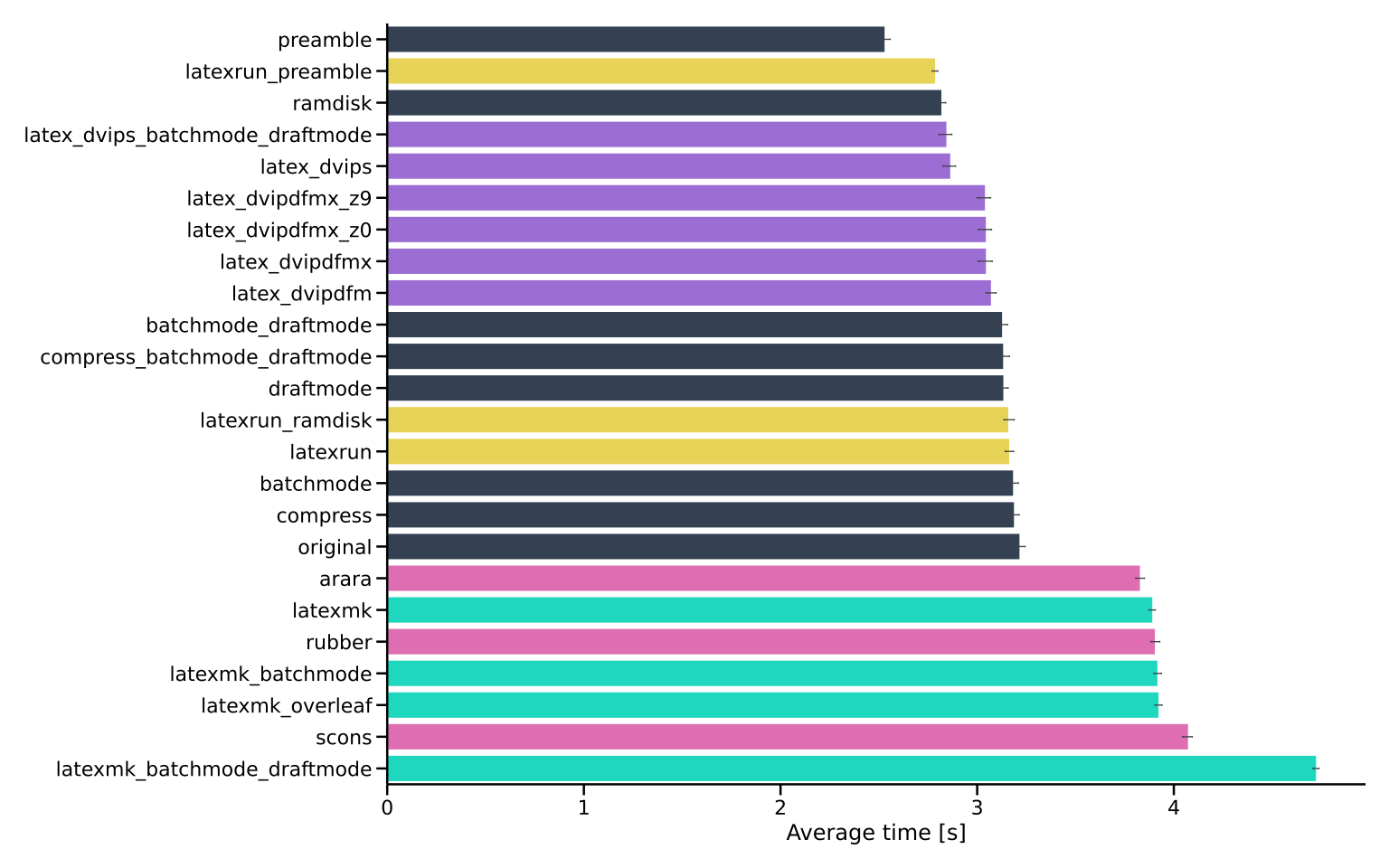
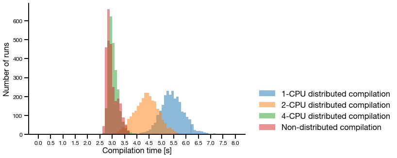
<p>Our most important metric, and the one we set out to measure, is the build time.
Faster build times improve the efficiency of the document creation process,
allowing you to iterate more quickly through drafts.  For those new to LaTeX, a
slow build process can be discouraging. Faster build times can make the learning
curve less steep. For me personally, long build times can interrupt my flow and
concentration, impacting overall productivity.</p>

<div class="container figure">
<div class="row">
    <div class="col-md-12">
        <div><img src="/assets/images/build_times.svg" alt="" /></div>
        <div class="caption">Build times</div>
    </div>
</div>
</div>

<p>In this figure we can see that the fastest build system is <code class="language-plaintext highlighter-rouge">preamble</code>, where we
precompile the preamble using <code class="language-plaintext highlighter-rouge">latex</code> and compile the rest of the document with
<code class="language-plaintext highlighter-rouge">latex+dvips+ps2pdf</code>. This speeds up the build a lot! In fact, in the first half
of the list we see a lot of the same type of pipeline.</p>

<h3 id="manageable-output">Manageable output</h3>

<p>Human-understandable output, especially during errors, is crucial in LaTeX
document building. Most of the information printed however, isn’t very useful,
so it would make sense to try and reduce this and keep the output to a minimum.
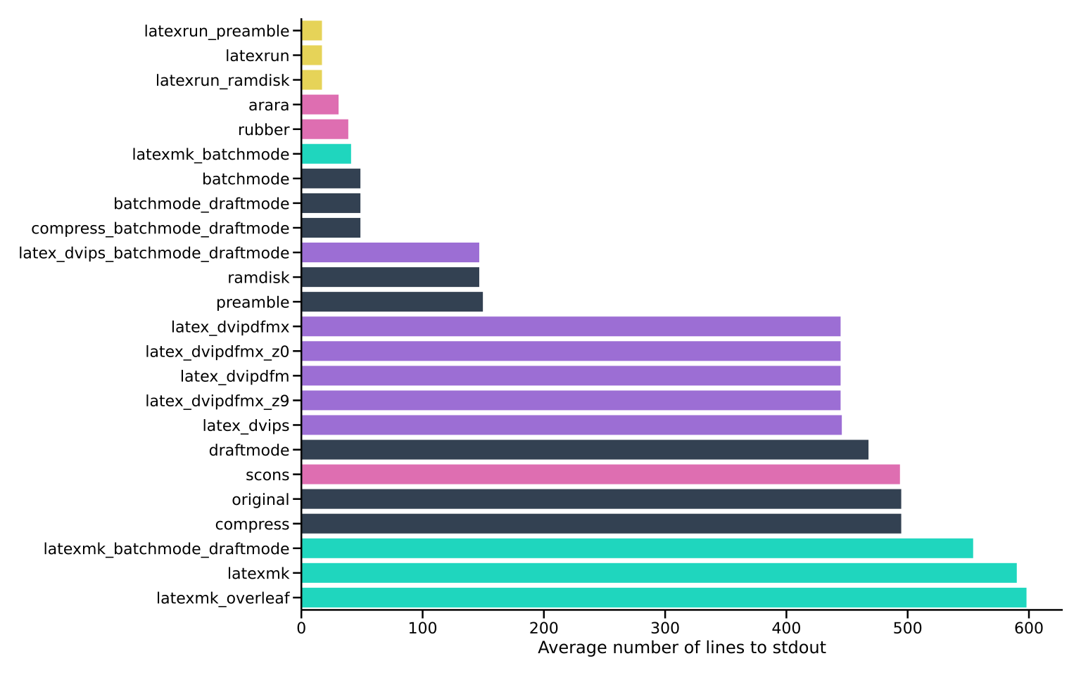
In this test we simply count the number of lines on <code class="language-plaintext highlighter-rouge">stdout</code>, but it should be
said that some of these build systems, such as <code class="language-plaintext highlighter-rouge">latexrun</code> have really nice
colored output in the case things do go wrong.</p>

<div class="container figure">
<div class="row">
    <div class="col-md-12">
        <div><img src="/assets/images/build_stdout.svg" alt="" /></div>
        <div class="caption">Number of lines printed to stdout.</div>
    </div>
</div>
</div>

<p>The first part of the list is dominated by build tools such as <code class="language-plaintext highlighter-rouge">latexrun</code>,
<code class="language-plaintext highlighter-rouge">arara</code> and <code class="language-plaintext highlighter-rouge">rubber</code>.</p>

<h3 id="ease-of-use">Ease of use</h3>

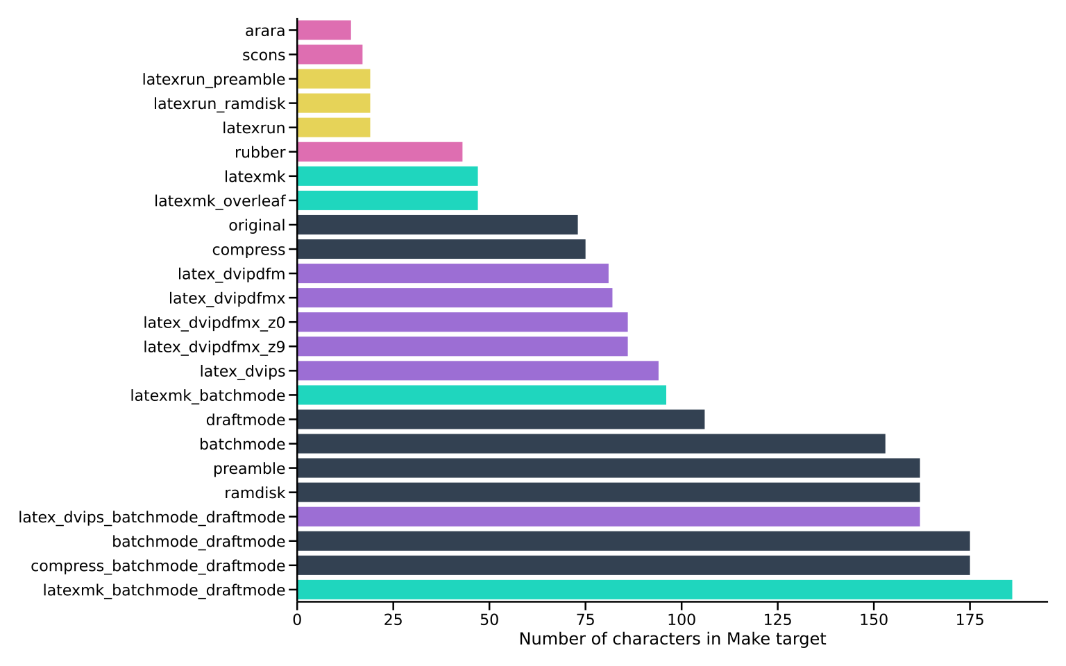
<p>A build system must of course be easy to use, and as a proxy for that we measure
the number of characters in the <code class="language-plaintext highlighter-rouge">Makefile</code> target. In the case that you do use a
<code class="language-plaintext highlighter-rouge">Makefile</code>, simply running <code class="language-plaintext highlighter-rouge">make</code> would of course be easy enough.</p>

<div class="container figure">
<div class="row">
    <div class="col-md-12">
        <div><img src="/assets/images/build_make.svg" alt="" /></div>
        <div class="caption">Number of lines in the Maketarget</div>
    </div>
</div>
</div>

<h3 id="file-size">File size</h3>

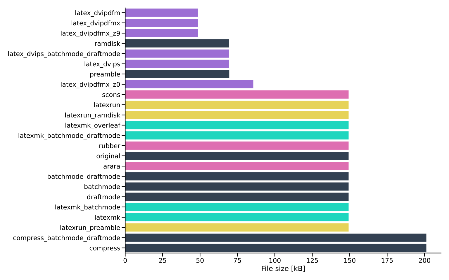
<p>A smaller file size offers advantages in terms of ease of handling, quicker
uploads, and efficient storage. Therefore, the file size serves as a crucial
parameter in evaluating performance.</p>

<div class="container figure">
<div class="row">    
    <div class="col-md-12">
        <div><img src="/assets/images/build_filesize.svg" alt="" /></div>
        <div class="caption">PDF file size</div>
    </div>
</div>
</div>

<p>It is interesting that there is such a big difference between the smallest and largest file size, even for such a simple document.</p>

<h3 id="final-score">Final score</h3>

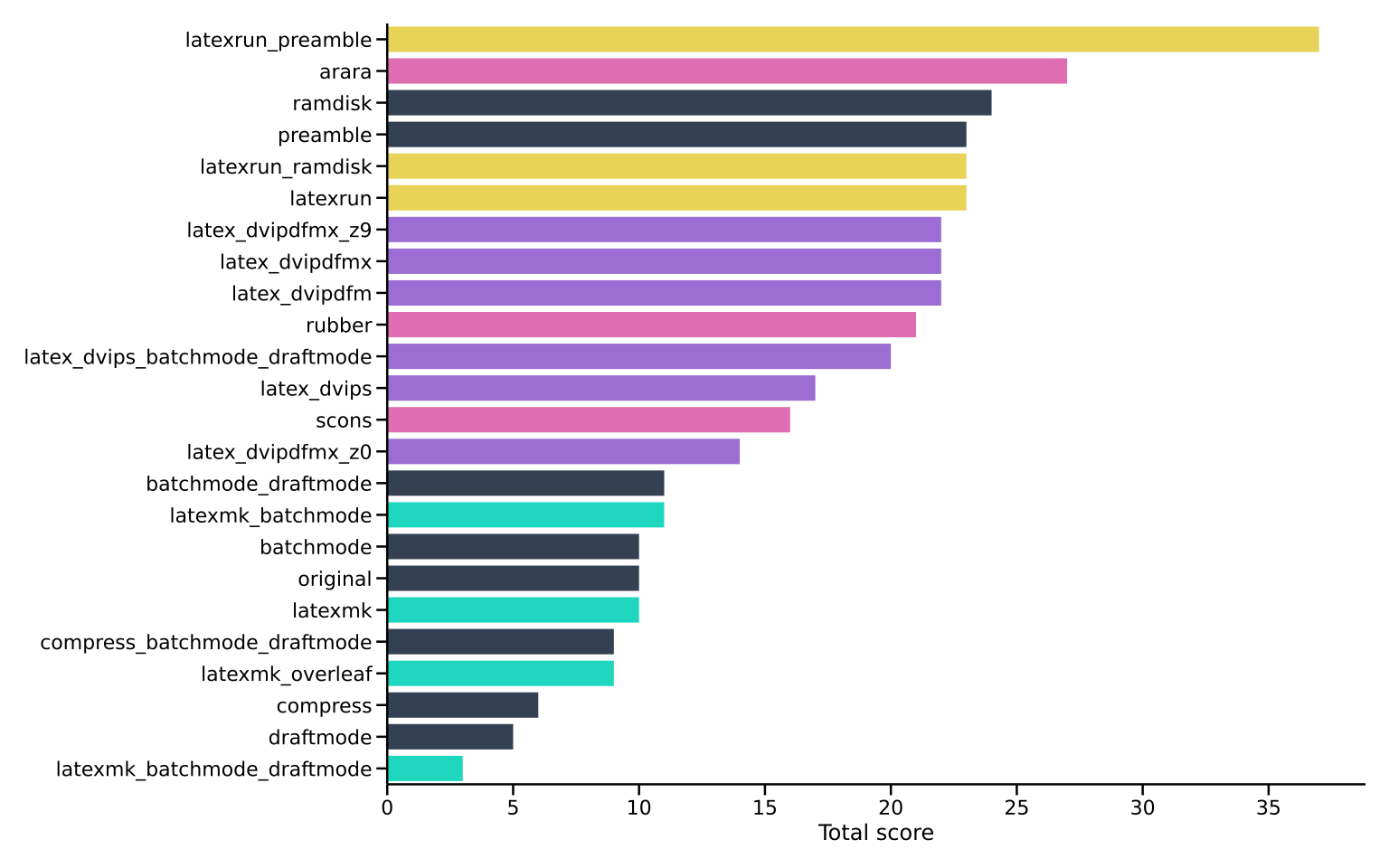
<p>In the spirit of Eurovision and Melodifestivalen, we will adopt a point
allocation system that mirrors the excitement and competition of these iconic
music events. In Eurovision, each participating country awards points to their
favorite songs, with the famous ‘douze points’ (12 points) reserved for the top
choice. Similarly, the runner-up receives 10 points, acknowledging outstanding
performances, and we will continue this tradition here.</p>

<div class="container figure">
<div class="row">
    <div class="col-md-12">
        <div><img src="/assets/images/build_scores.svg" alt="" /></div>
        <div class="caption">Total scores received.</div>
    </div>
</div>
</div>

<p>The build system with the greatest final score is <code class="language-plaintext highlighter-rouge">latexrun</code>. We have seen how
we can improve the compilation time for a small toy project, but these
improvements carry over to real documents as well. For example, compiling a
recent IEEE paper using <code class="language-plaintext highlighter-rouge">latexrun</code> took 16.87 seconds compared to 25.71 seconds
using <code class="language-plaintext highlighter-rouge">latexmk</code>.</p>

<h2 id="related-work">Related work</h2>

<p>There are many general build systems such as Snakemake <a class="citation" href="#Koster2012">(Koster &amp; Rahmann, 2012)</a>,
GNU Make, CMake, etc that can be used also to build LaTeX documents. There are
also many LaTeX specific build systems such as
<a href="https://awmacpherson.com/posts/make-latex/">make-latex</a>,
<a href="https://www.arakhne.org/autolatex/">AutoLaTeX</a> and
<a href="https://github.com/reitzig/ltx2any">ltx2any</a>, that didn’t make it into this
comparison for one reason or another and I hope to return to them at a later
date.</p>

<p>Each of these tools can be use in a more general pipeline as explored in <a href="/2020/05/11/gitlab-ci-latex-pipeline/">How to
annoy your co-authors: a Gitlab CI pipeline for LaTeX </a>.</p>

<p>If you have many TikZ <a class="citation" href="#Tikz2014">(Feuersänger et al., 2014; Tantau, 2007)</a> or pgfplots <a class="citation" href="#Feuersanger2014">(Feuersänger, 2014)</a> figures, it might be worthwhile to externalize them <a class="citation" href="#wenneker2012_tikz">(Wenneker, 2012)</a>.</p>

<h2 id="discussion-and-limitations">Discussion and limitations</h2>

<p>In this blog post, we have strived to cover the most common build systems and
tool combinations for LaTeX document compilation. These systems have been chosen
based on their popularity and widespread use within the LaTeX community.
However, it’s important to recognize that the world of LaTeX is vast, and new
tools and approaches are continually emerging.</p>

<p>Therefore, one obvious limitation of this blog post is its inevitable inability
to encompass every possible LaTeX build system and tool combination. The LaTeX
ecosystem is dynamic, with developers and enthusiasts constantly devising
innovative ways to streamline the document creation process. As a result, there
may be niche or specialized tools that we have not explored here.</p>

<p>Some characteristics of a build system might be more important to you. For
example, the output from  <code class="language-plaintext highlighter-rouge">latexrun</code> in the case of a fault is much easier to
read than for other build systems, and it leaves a build directory that is
almost clean. However, build directory cleanness is not measured in this blog
post.</p>

<p>Your choice of a LaTeX build system should of course be guided by your
individual preferences and workflow requirements. For example, when selecting a
build system, consider factors such as your operating system and LaTeX
distribution. Some tools are more compatible with specific platforms, and this
compatibility restricts what options are available to you.</p>

<h2 id="conclusion">Conclusion</h2>

<p>In the realm of LaTeX document compilation, where efficiency and reliability are
paramount, one contender stands out as the victor – <code class="language-plaintext highlighter-rouge">latexrun</code> when precompiling
the preamble. Through our exploration of various build systems, including
<code class="language-plaintext highlighter-rouge">latexmk</code>, <code class="language-plaintext highlighter-rouge">arara</code>, SCons, and <code class="language-plaintext highlighter-rouge">latexrun</code>, it becomes clear that <code class="language-plaintext highlighter-rouge">latexrun</code>
in any of our variations stand out as a very good build system.</p>

<p>In the ever-evolving landscape of LaTeX document compilation, choosing the right
build system is a critical decision. While each contender we explored has its
strengths, <code class="language-plaintext highlighter-rouge">latexrun</code> emerges as the true champion, combining efficiency,
reproducibility, and versatility in a single package. As you embark on your
document creation journey, consider embracing <code class="language-plaintext highlighter-rouge">latexrun</code> as your reliable ally
in crafting elegant and polished documents, all while reclaiming precious time
and focus for what truly matters – your content.</p>]]></content><author><name>Martin Isaksson</name><email>martin@martisak.se</email></author><category term="academia" /><category term="latex" /><category term="latex" /><summary type="html"><![CDATA[Long LaTeX build times can be a significant challenge for researchers and developers, hampering productivity and efficiency. This issue arises due to the complexity of LaTeX documents and the diversity of build systems available. We present a comprehensive exploration of LaTeX build systems, helping authors choose the most suitable one. By identifying the best build system, authors can streamline their workflow, reduce build times, and ultimately enhance their research and development endeavors.]]></summary><media:thumbnail xmlns:media="http://search.yahoo.com/mrss/" url="https://blog.martisak.se/images/blog-4.jpg" /><media:content medium="image" url="https://blog.martisak.se/images/blog-4.jpg" xmlns:media="http://search.yahoo.com/mrss/" /></entry><entry><title type="html">Top LaTeX commands and macros for academic writing (and more)</title><link href="https://blog.martisak.se/2023/08/11/top-latex-commands/" rel="alternate" type="text/html" title="Top LaTeX commands and macros for academic writing (and more)" /><published>2023-08-11T00:00:00+00:00</published><updated>2023-08-11T00:00:00+00:00</updated><id>https://blog.martisak.se/2023/08/11/top-latex-commands</id><content type="html" xml:base="https://blog.martisak.se/2023/08/11/top-latex-commands/"><![CDATA[<p><strong>LaTeX, a typesetting system celebrated for its capacity to effortlessly blend
visual appeal with practicality, remains an essential instrument for both
researchers and academics. While its inherent capabilities are impressive, the
full potential of LaTeX is revealed through the skillful utilization of its
macros. As a researcher in the field of artificial intelligence, I find that I
am very often using a set of LaTeX commands, macros and definitions when writing
academic papers, and perhaps you will find them useful too.</strong></p>

<!--more-->

<h2 id="introduction">Introduction</h2>

<p>In this blog post, we embark on a journey through the realm of LaTeX macros,
unveiling the <del>ten</del> eighteen most essential ones tailored specifically to
elevate your computer science paper writing endeavors. From effortlessly
formatting algorithms to seamlessly managing references, these macros are poised
to revolutionize your writing process, empowering you to focus more on your
content and less on formatting intricacies. Whether you’re a seasoned LaTeX user
or just beginning to explore its capabilities, this compilation promises to
enhance your efficiency, organization, and overall output in the domain of
computer science research.</p>

<p>In an <a href="/2020/05/03/top-ten-latex-packages/">earlier post</a> we had a
look at ten LaTeX packages, but in this post we will look at commands and
macros. So, without further ado, and in no particular order, here are <del>10</del> 18
useful LaTeX commands, macros and other tips for your writing pleasure.</p>

<h2 id="commands-macros-and-other-tips">Commands, macros and other tips</h2>

<h3 id="math-modes">Math modes</h3>

<p>When writing math in a paper, you can the LaTeX syntax <code class="language-plaintext highlighter-rouge">\( x = 1 \)</code> (or <code class="language-plaintext highlighter-rouge">\[</code>
for inline math mode <a class="citation" href="#wright_math_2022">(Wright, 2022)</a>. This will sometimes provide
better error messages, and having a begin and end point is nice if you ever
would like to parse the document with a script. The TeX
syntax <code class="language-plaintext highlighter-rouge">$ x = 1 $</code> works as well, and some will say that this is more readable.
Read about other subtle differences at <i class="ai ai-stackoverflow-square"></i> <a href="https://tex.stackexchange.com/questions/510/are-and-preferable-to-dollar-signs-for-math-mode.">Are \ ( and \ ) preferable to dollar signs
for math
mode?</a></p>

<p>It is common that LaTeX introduces a line break inside the equation, which might
not look great for inline math. You can use curly brackets to avoid the line
breaking, for example <code class="language-plaintext highlighter-rouge">\({ x = 1 }\)</code>.</p>

<h3 id="dynamic-delimiters">Dynamic delimiters</h3>

<p>Dynamic delimiters in LaTeX are great because they automatically adjust their size to match the content they enclose, ensuring optimal readability and aesthetic presentation of mathematical expressions.</p>

<p>You <em>can</em> manually vary the size of delimiters such as parentheses with <code class="language-plaintext highlighter-rouge">\big(</code>, <code class="language-plaintext highlighter-rouge">\Big(</code>,
<code class="language-plaintext highlighter-rouge">\bigg(</code> and <code class="language-plaintext highlighter-rouge">\Bigg(</code>.</p>

\[( \bigl( \Bigl( \biggl( \Biggl(\]

<p>However, almost always I use dynamically sized delimiters.</p>

<figure class="highlight"><pre><code class="language-tex" data-lang="tex"><table class="rouge-table"><tbody><tr><td class="gutter gl"><pre class="lineno">1
</pre></td><td class="code"><pre><span class="k">\left</span>( <span class="k">\sqrt</span><span class="p">{</span>a<span class="p">}</span>+<span class="k">\sqrt</span><span class="p">{</span>b<span class="p">}</span><span class="k">\right</span> )<span class="p">^</span>2
</pre></td></tr></tbody></table></code></pre></figure>

<p>which produces</p>

\[\left( \sqrt{a}+\sqrt{b} \right)^2\]

<p>as opposed to</p>

\[( \sqrt{a}+\sqrt{b} )^2\]

<p>without using <code class="language-plaintext highlighter-rouge">\left(</code> and <code class="language-plaintext highlighter-rouge">\right)</code>.</p>

<p>I recently learned we can do even better by declaring paired delimiters <a class="citation" href="#zeng_2023_art">(Zeng, 2023)</a>! By using the <code class="language-plaintext highlighter-rouge">mathtools</code> <a class="citation" href="#madsen2022">(Madsen et al., 2022)</a> package we can define a paired braces with</p>

<figure class="highlight"><pre><code class="language-tex" data-lang="tex"><table class="rouge-table"><tbody><tr><td class="gutter gl"><pre class="lineno">1
</pre></td><td class="code"><pre><span class="k">\DeclarePairedDelimiter\braces</span><span class="p">{</span><span class="k">\lbrace</span><span class="p">}{</span><span class="k">\rbrace</span><span class="p">}</span>
</pre></td></tr></tbody></table></code></pre></figure>

<p>Then we can use the command <code class="language-plaintext highlighter-rouge">\braces*{ ...}</code> (note the starred version here) <a class="citation" href="#zeng_2023_art">(Zeng, 2023)</a>.</p>

<p>Read more about brackets, parantheses and scaling the middle vertical line in <i class="ai ai-overleaf-square"></i> <a href="https://www.overleaf.com/learn/latex/Brackets_and_Parentheses">Brackets and Parentheses</a> and
<i class="ai ai-stackoverflow-square"></i> <a href="https://tex.stackexchange.com/questions/108388/how-to-automatically-scale-mid-within-delimiters">How to automatically scale <code class="language-plaintext highlighter-rouge">\mid</code> within delimiters</a>. Read more about declaring paired delimiters at <i class="ai ai-overleaf-square"></i> <a href="https://tex.stackexchange.com/questions/1742/automatic-left-and-right-commands/">Automatic left and right commands</a>.</p>

<h3 id="numbers-and-units">Numbers and units</h3>

<p><code class="language-plaintext highlighter-rouge">siunitx</code> <a class="citation" href="#Wright2009">(Wright, 2009)</a> is a powerful tool for typesetting and formatting scientific and technical documents. It specializes in handling units, quantities, and numerical values, ensuring proper spacing, alignment, and consistent appearance.</p>

<figure class="highlight"><pre><code class="language-tex" data-lang="tex"><table class="rouge-table"><tbody><tr><td class="gutter gl"><pre class="lineno">1
2
3
4
5
6
7
8
9
10
11
12
</pre></td><td class="code"><pre><span class="k">\usepackage</span><span class="p">{</span>siunitx<span class="p">}</span>

<span class="c">% SI unit setup</span>
<span class="k">\sisetup</span><span class="p">{</span>
    load-configurations = abbreviations,
    binary-units = true,
    exponent-product=<span class="k">\cdot</span>
<span class="p">}</span>

<span class="k">\DeclareSIUnit</span><span class="p">{</span><span class="k">\belmilliwatt</span><span class="p">}{</span>Bm<span class="p">}</span>
<span class="k">\DeclareSIUnit</span><span class="p">{</span><span class="k">\dBm</span><span class="p">}{</span><span class="k">\deci\belmilliwatt</span><span class="p">}</span>
<span class="k">\DeclareSIUnit\px</span><span class="p">{</span>px<span class="p">}</span>
</pre></td></tr></tbody></table></code></pre></figure>

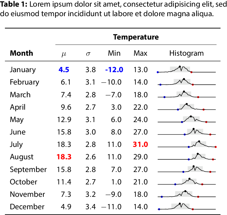
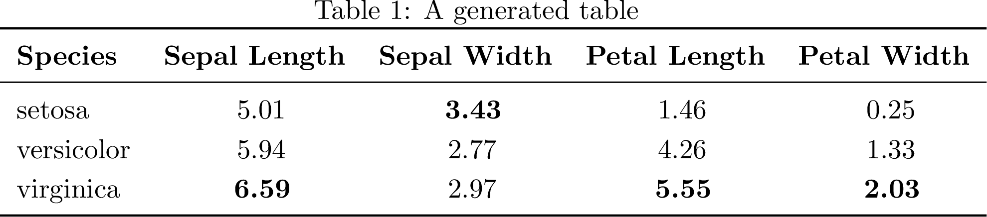
<p>This allows us to add a number and unit with <code class="language-plaintext highlighter-rouge">\SI{52}{\ampere\meter}</code>. A number can be typeset with <code class="language-plaintext highlighter-rouge">\num{1e5}</code>. In an <a href="/2021/04/10/publication_ready_tables/">earlier post</a>, we looked at using Pandas <a class="citation" href="#reback2020pandas">(pandas development team, 2020; Wes McKinney, 2010 )</a> to produce nice looking tables with no manual steps, and here we also used the table format <code class="language-plaintext highlighter-rouge">S</code> from <code class="language-plaintext highlighter-rouge">siunitx</code>.</p>

<h3 id="spaces-and-domains">Spaces and domains</h3>

<p>Here are a few definitions of domains that I use.</p>

<figure class="highlight"><pre><code class="language-tex" data-lang="tex"><table class="rouge-table"><tbody><tr><td class="gutter gl"><pre class="lineno">1
2
3
4
5
</pre></td><td class="code"><pre><span class="k">\newcommand</span><span class="p">{</span><span class="k">\Z</span><span class="p">}{</span><span class="k">\mathbb</span><span class="p">{</span>Z<span class="p">}}</span> <span class="c">% Integer numbers</span>
<span class="k">\newcommand</span><span class="p">{</span><span class="k">\R</span><span class="p">}{</span><span class="k">\mathbb</span><span class="p">{</span>R<span class="p">}}</span> <span class="c">% Real numbers</span>
<span class="k">\newcommand</span><span class="p">{</span><span class="k">\N</span><span class="p">}{</span><span class="k">\mathbb</span><span class="p">{</span>N<span class="p">}}</span> <span class="c">% Natural numbers or prime numbers</span>
<span class="k">\newcommand</span><span class="p">{</span><span class="k">\C</span><span class="p">}{</span><span class="k">\mathbb</span><span class="p">{</span>C<span class="p">}}</span> <span class="c">% Complex numbers</span>
<span class="k">\newcommand</span><span class="p">{</span><span class="k">\Np</span><span class="p">}{</span><span class="k">\mathbb</span><span class="p">{</span>N<span class="p">}^</span>+<span class="p">}</span> <span class="c">% Natural numbers including 0</span>
</pre></td></tr></tbody></table></code></pre></figure>

<p>For example <code class="language-plaintext highlighter-rouge">\mathbb{N}^+ = \mathbb{N} \setminus \{0\}</code> \(\mathbb{N}^+ = \mathbb{N} \setminus \{0\}\). To denote the empty set, I prefer <code class="language-plaintext highlighter-rouge">$\varnothing</code> \(\varnothing\) over <code class="language-plaintext highlighter-rouge">\emptyset</code> \(\emptyset\). For this, and many many more notations, see <a class="citation" href="#siek_latex_formal">(Siek, n.d.)</a>.</p>

<h3 id="bachmann-landau-notations">Bachmann-Landau notations</h3>

<p>Bachmann-Landau notation, a fundamental concept in theoretical computer science and mathematics, offers a concise and standardized way to describe the growth rates of functions and their relationships in mathematical analysis. Named after the mathematicians Paul Bachmann and Edmund Landau <a class="citation" href="#enwiki:1168125072">(Wikipedia contributors, 2023)</a>, this notation employs symbols like \(\mathcal{O}\), \(\Omega\), \(\Theta\), \(o\), \(\omega\) and \(\sim\) to articulate upper, lower, and tight bounds, on the behavior of functions as their inputs become sufficiently large. Bachmann-Landau notation provides a powerful tool for comparing algorithmic efficiencies, predicting performance, and understanding the scalability of mathematical models and algorithms.</p>

<p>Put this in your document preamble.</p>

<figure class="highlight"><pre><code class="language-tex" data-lang="tex"><table class="rouge-table"><tbody><tr><td class="gutter gl"><pre class="lineno">1
2
</pre></td><td class="code"><pre><span class="k">\usepackage</span><span class="p">{</span>amssymb<span class="p">}</span>
<span class="k">\newcommand</span><span class="p">{</span><span class="k">\BigO</span><span class="p">}</span>[1]<span class="p">{</span><span class="k">\mathcal</span><span class="p">{</span>O<span class="p">}</span><span class="k">\!\left</span>(#1<span class="k">\right</span>)<span class="p">}</span>
</pre></td></tr></tbody></table></code></pre></figure>

<p>Then we can you the command ´\BigO{}` like this:</p>

<figure class="highlight"><pre><code class="language-tex" data-lang="tex"><table class="rouge-table"><tbody><tr><td class="gutter gl"><pre class="lineno">1
</pre></td><td class="code"><pre><span class="k">\BigO</span><span class="p">{</span>n<span class="k">\log</span><span class="p">{}</span>n<span class="p">}</span>
</pre></td></tr></tbody></table></code></pre></figure>

<p>This will produce \(\mathcal{O}\!\left(n \log{n}\right)\). Here is a <a href="https://texblog.org/2014/06/24/big-o-and-related-notations-in-latex">Complete list of Bachmann-Landau notations</a>. The <code class="language-plaintext highlighter-rouge">\!</code> adjusts the spacing to be more pleasing (Thanks <a href="https://www.reddit.com/user/Tensor_Product_9377/">u/Tensor_Product_9377</a>!).</p>

<h3 id="defining-new-math-operators">Defining new math operators</h3>

<p>Operators such as \(\sin\) and \(\cos\) are typeset in a roman font in math mode <a class="citation" href="#nhigham_top_tips">(Higham, n.d.)</a>
. If you need to define a new operator, you can use <code class="language-plaintext highlighter-rouge">amsmath</code> to make sure spacing is consistent with the already defined operators.</p>

<figure class="highlight"><pre><code class="language-tex" data-lang="tex"><table class="rouge-table"><tbody><tr><td class="gutter gl"><pre class="lineno">1
2
3
4
5
6
7
8
9
10
11
</pre></td><td class="code"><pre><span class="k">\usepackage</span><span class="p">{</span>amsmath<span class="p">}</span>
<span class="k">\DeclareMathOperator</span><span class="p">{</span><span class="k">\tr</span><span class="p">}{</span>tr<span class="p">}</span>
<span class="k">\DeclareMathOperator*</span><span class="p">{</span><span class="k">\Max</span><span class="p">}{</span>Max<span class="p">}</span>
<span class="k">\DeclareMathOperator</span><span class="p">{</span><span class="k">\Prob</span><span class="p">}{</span><span class="k">\mathcal</span><span class="p">{</span>P<span class="p">}}</span>
<span class="k">\DeclareMathOperator</span><span class="p">{</span><span class="k">\sgn</span><span class="p">}{</span>sgn<span class="p">}</span>
<span class="k">\DeclareMathOperator</span><span class="p">{</span><span class="k">\DFT</span><span class="p">}{</span>DFT<span class="p">}</span>

<span class="nt">\begin{displaymath}</span>
  <span class="k">\Max</span><span class="p">_{</span>x<span class="k">\in</span> A<span class="p">}</span> f(x) <span class="k">\qquad</span>  <span class="k">\End</span><span class="p">_</span>R V 
<span class="nt">\end{displaymath}</span>
<span class="k">\def\diag</span><span class="p">{</span><span class="k">\mathop</span><span class="p">{</span><span class="k">\mathrm</span><span class="p">{</span>diag<span class="p">}}}</span>
</pre></td></tr></tbody></table></code></pre></figure>

<p>See <i class="ai ai-stackoverflow-square"></i> <a href="https://tex.stackexchange.com/questions/67506/newcommand-vs-declaremathoperator">newcommand vs. DeclareMathOperator</a> and 
<a href="https://texfaq.org/FAQ-newfunction">Defining a new log-like function in LaTeX</a> for more information.</p>

<h3 id="typesetting-a-definition">Typesetting a definition</h3>

<p>Sometimes I see the notation <code class="language-plaintext highlighter-rouge">:=</code> to denote a definition, and I don’t particularily care for it. I much prefer the overset triangle <code class="language-plaintext highlighter-rouge">\triangleq</code> \(\triangleq\) from <code class="language-plaintext highlighter-rouge">amssymb</code>.</p>

<p>If you’d rather use an overset text <code class="language-plaintext highlighter-rouge">def</code>, here is how to do that.</p>

<figure class="highlight"><pre><code class="language-tex" data-lang="tex"><table class="rouge-table"><tbody><tr><td class="gutter gl"><pre class="lineno">1
</pre></td><td class="code"><pre><span class="k">\newcommand\myeq</span><span class="p">{</span><span class="k">\mathrel</span><span class="p">{</span><span class="k">\overset</span><span class="p">{</span><span class="k">\makebox</span><span class="na">[0pt]</span><span class="p">{</span><span class="k">\mbox</span><span class="p">{</span><span class="k">\normalfont\tiny\sffamily</span> def<span class="p">}}}{</span>=<span class="p">}}}</span>
</pre></td></tr></tbody></table></code></pre></figure>

<div class="container figure">
<div class="row">
    <div class="col-md-4">
        <div><img src="/assets/images/def.png" alt="" /></div>
        <div class="caption">Overset text</div>
    </div>
    <div class="col-md-4">
        <div><img src="/assets/images/def_tri.png" alt="" /></div>
        <div class="caption"><code>amssymb</code></div>
    </div>
</div>
</div>

<p>See <i class="ai ai-stackoverflow-square"></i> <a href="https://tex.stackexchange.com/questions/523097/triangle-on-top-of-propto-that-matches-triangleq">Triangle on top of propto that matches \triangleq</a>, <i class="ai ai-stackoverflow-square"></i> <a href="https://math.stackexchange.com/questions/450175/notation-for-definition-and-equivalence">Notation for definition and equivalence</a>, <i class="ai ai-stackoverflow-square"></i> <a href="https://tex.stackexchange.com/questions/74125/how-do-i-put-text-over-symbols">How do I put text over symbols?</a> and
<i class="ai ai-stackoverflow-square"></i> <a href="https://tex.stackexchange.com/questions/163829/delta-equal-to-symbol">Delta-equal to symbol</a>
 for more information on the topic.</p>

<h3 id="vectors-and-matrices">Vectors and matrices</h3>

<p>When I studied physics, my preferred way of writing vectors was using <code class="language-plaintext highlighter-rouge">\vec{x}</code> \(\vec{x}\). Nowadays, I prefer to use bold symbols for vectors and matrices using the <code class="language-plaintext highlighter-rouge">bm</code> package <code class="language-plaintext highlighter-rouge">\bm{x}</code> \(\bm{x}\).</p>

<p>See <i class="ai ai-stackoverflow-square"></i> <a href="https://tex.stackexchange.com/questions/3238/bm-package-versus-boldsymbol">bm package versus \boldsymbol</a> for more information.</p>

<h3 id="transpose-symbol">Transpose symbol</h3>

<p>Here is a controversial topic on which transpose sign to use. I prefer <code class="language-plaintext highlighter-rouge">\intercal</code> over <code class="language-plaintext highlighter-rouge">T</code> any day of the week, but I agree with the user <a href="https://tex.stackexchange.com/users/16967/heiko-oberdiek">@Heiko Oberdiek</a> that it is typeset a little too low for capital symbols (such as matrices). For lowercase symbols, just using <code class="language-plaintext highlighter-rouge">\intercal</code> looks better to me. See the full discussion on <i class="ai ai-stackoverflow-square"></i> <a href="https://tex.stackexchange.com/questions/30619/what-is-the-best-symbol-for-vector-matrix-transpose">What is the best symbol for vector/matrix transpose?</a>.</p>

<figure class="highlight"><pre><code class="language-tex" data-lang="tex"><table class="rouge-table"><tbody><tr><td class="gutter gl"><pre class="lineno">1
2
3
4
</pre></td><td class="code"><pre><span class="k">\makeatletter</span>
<span class="k">\newcommand*</span><span class="p">{</span><span class="k">\transpose</span><span class="p">}}</span>
<span class="k">\newcommand*</span><span class="p">{</span><span class="k">\@</span>transpose<span class="p">}</span>[2]<span class="p">{</span><span class="k">\raisebox</span><span class="p">{</span><span class="k">\depth</span><span class="p">}{$</span><span class="nv">\m</span><span class="nb">@th#</span><span class="m">1</span><span class="nv">\intercal</span><span class="p">$}}</span>
<span class="k">\makeatother</span>
</pre></td></tr></tbody></table></code></pre></figure>

<div class="row justify-content-md-center figure ">
    <div class="col-md-3">
        <div class="">
            <img src="/assets/images/transpose.png" alt="Transpose example" />
        </div>
        <div class="caption">Transpose example</div>
    </div>
</div>

<p>I would like to have one macro for both lowercase and for uppercase symbols alike.</p>

<h3 id="overbrackets-and-underbrackets">Overbrackets and underbrackets</h3>

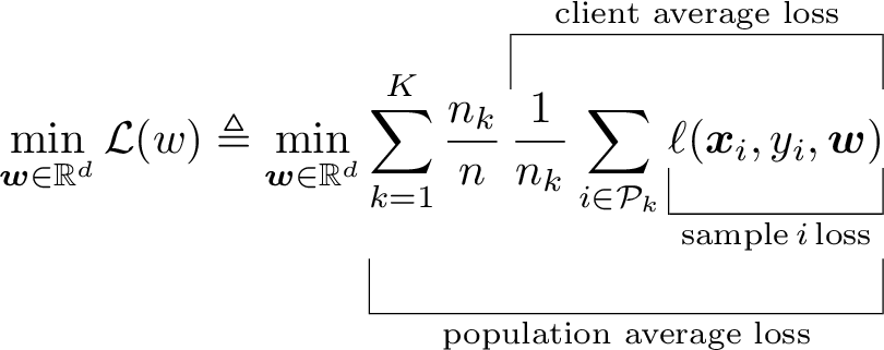
<p>Brackets, and braces, provide an excellent way of highlighting a part of an equation to be able to explain in better.</p>

<figure class="highlight"><pre><code class="language-tex" data-lang="tex"><table class="rouge-table"><tbody><tr><td class="gutter gl"><pre class="lineno">1
2
3
</pre></td><td class="code"><pre><span class="nt">\begin{equation}</span>
    <span class="k">\min</span><span class="p">_{</span><span class="k">\bm</span><span class="p">{</span>w<span class="p">}</span> <span class="k">\in</span> <span class="k">\mathbb</span><span class="p">{</span>R<span class="p">}^</span>d<span class="p">}</span> <span class="k">\mathcal</span><span class="p">{</span>L<span class="p">}</span>(w) <span class="k">\triangleq</span> <span class="k">\min</span><span class="p">_{</span><span class="k">\bm</span><span class="p">{</span>w<span class="p">}</span> <span class="k">\in</span> <span class="k">\mathbb</span><span class="p">{</span>R<span class="p">}^</span>d<span class="p">}</span> <span class="k">\underbracket</span><span class="na">[.25pt][12pt]</span><span class="p">{</span><span class="k">\sum</span><span class="p">_{</span>k=1<span class="p">}^</span>K <span class="k">\frac</span><span class="p">{</span>n<span class="p">_</span>k<span class="p">}{</span>n<span class="p">}</span> <span class="k">\overbracket</span><span class="na">[.25pt][12pt]</span><span class="p">{</span><span class="k">\frac</span><span class="p">{</span>1<span class="p">}{</span>n<span class="p">_</span>k<span class="p">}</span> <span class="k">\sum</span><span class="p">_{</span>i <span class="k">\in</span> <span class="k">\mathcal</span><span class="p">{</span>P<span class="p">}_</span>k<span class="p">}</span>  <span class="k">\underbracket</span><span class="na">[.25pt][10pt]</span><span class="p">{</span><span class="k">\ell</span>(<span class="k">\bm</span><span class="p">{</span>x<span class="p">}_</span>i, y<span class="p">_</span>i, <span class="k">\bm</span><span class="p">{</span>w<span class="p">}</span>)<span class="p">}_{</span><span class="k">\text</span><span class="p">{</span>sample<span class="p">}</span><span class="k">\,</span>i<span class="k">\,\text</span><span class="p">{</span>loss<span class="p">}}}^{</span><span class="k">\text</span><span class="p">{</span>client average loss<span class="p">}}}_{</span><span class="k">\text</span><span class="p">{</span>population average loss<span class="p">}}</span>
<span class="nt">\end{equation}</span>
</pre></td></tr></tbody></table></code></pre></figure>

<div class="row justify-content-md-center figure ">
    <div class="col-md-6">
        <div class="">
            <img src="/assets/images/brackets.png" alt="Under and over-brackets example" />
        </div>
        <div class="caption">Under and over-brackets example</div>
    </div>
</div>

<h3 id="inline-tikz">Inline TikZ</h3>

<p>Sometimes it is easier to explain something with a small figure instead of creating some notation that is difficult to understand. I like to use this in a figure caption for example. We can use the <code class="language-plaintext highlighter-rouge">tikz</code> package <a class="citation" href="#Tikz2014">(Feuersänger et al., 2014)</a> for this.</p>

<figure class="highlight"><pre><code class="language-tex" data-lang="tex"><table class="rouge-table"><tbody><tr><td class="gutter gl"><pre class="lineno">1
2
3
4
5
6
7
8
9
10
</pre></td><td class="code"><pre><span class="k">\documentclass</span><span class="na">[varwidth=true, border=0pt, convert={outext=.png}]</span><span class="p">{</span>standalone<span class="p">}</span>
<span class="k">\usepackage</span><span class="p">{</span>tikz<span class="p">}</span>
<span class="k">\usepackage</span><span class="p">{</span>xcolor<span class="p">}</span>
<span class="k">\newcommand</span><span class="p">{</span><span class="k">\sharedkey</span><span class="p">}{</span>
    <span class="k">\raisebox</span><span class="p">{</span>-.5 ex<span class="p">}{</span><span class="k">\tikz</span><span class="p">{</span>
    <span class="k">\draw</span><span class="na">[fill=blue, draw=white]</span> (0ex,0) arc(90:270:1ex) -- cycle;
    <span class="k">\draw</span><span class="na">[fill=red, draw=white]</span> (0ex,0) arc(90:-90:1ex) -- cycle; <span class="p">}}}</span>
<span class="nt">\begin{document}</span>
<span class="p">\(</span><span class="nb">x </span><span class="o">=</span><span class="nb"> </span><span class="nv">\sharedkey</span><span class="p">\)</span>
<span class="nt">\end{document}</span>
</pre></td></tr></tbody></table></code></pre></figure>

<div class="row justify-content-md-center figure ">
    <div class="col-md-3">
        <div class="">
            <img src="/assets/images/tikzmwe.png" alt="Inline TikZ example" />
        </div>
        <div class="caption">Inline TikZ example</div>
    </div>
</div>

<p>See <i class="ai ai-stackoverflow-square"></i> <a href="https://tex.stackexchange.com/questions/313927/tikz-picture-inline">Tikz picture inline</a> for some other examples.</p>

<h3 id="figure-up-top">Figure up top</h3>

<p>It is advantageous to put a nice overview figure in the top right corner <a class="citation" href="#Huang2018">(Huang, 2018)</a>, but it can be a bit fiddly to do so. From <i class="ai ai-stackoverflow-square"></i> <a href="https://tex.stackexchange.com/questions/63131/start-placing-figures-on-right-hand-side-column-of-first-page">StackExchange: Start placing figures on right-hand side column of first page</a> we learn a trick that makes it easier!</p>

<figure class="highlight"><pre><code class="language-tex" data-lang="tex"><table class="rouge-table"><tbody><tr><td class="gutter gl"><pre class="lineno">1
2
3
4
5
6
7
8
9
10
11
12
13
14
15
16
17
18
19
20
21
22
23
24
25
</pre></td><td class="code"><pre><span class="k">\documentclass</span><span class="p">{</span>IEEEtran<span class="p">}</span>
<span class="k">\usepackage</span><span class="p">{</span>lipsum<span class="p">}</span>

<span class="k">\title</span><span class="p">{</span>My IEEE article<span class="p">}</span>
<span class="k">\author</span><span class="p">{</span>Author<span class="p">}</span>

<span class="nt">\begin{document}</span>
<span class="k">\maketitle</span>
<span class="k">\global\csname</span> @topnum<span class="k">\endcsname</span> 0
<span class="k">\global\csname</span> @botnum<span class="k">\endcsname</span> 0
<span class="nt">\begin{abstract}</span> <span class="k">\lipsum</span><span class="na">[1]</span><span class="nt">\end{abstract}</span>

<span class="k">\section</span><span class="p">{</span>First Section<span class="p">}</span>

As you can see in Fig~<span class="k">\ref</span><span class="p">{</span>fig<span class="p">}</span>

<span class="nt">\begin{figure}</span>
<span class="k">\centering</span>
<span class="k">\fbox</span><span class="p">{</span>A nice figure<span class="p">}</span>
<span class="k">\caption</span><span class="p">{</span>A nice figure<span class="p">}</span><span class="k">\label</span><span class="p">{</span>fig<span class="p">}</span>
<span class="nt">\end{figure}</span>

<span class="k">\lipsum</span><span class="na">[1-5]</span>

<span class="nt">\end{document}</span>
</pre></td></tr></tbody></table></code></pre></figure>

<div class="row justify-content-md-center figure">
    <div class="col-md-6">
        <div class="papers">
            <img src="/assets/images/ieee-figure-without-0.png" alt="Without code, figure is in the left column." class="img-fluid" />
        </div>
        <div class="caption">Without</div>
    </div>
    
    <div class="col-md-6">
        <div class="papers">
            <img src="/assets/images/ieee-figure-with-0.png" alt="With code, figure is in the right column." class="img-fluid" />
        </div>
        <div class="caption">With</div>
    </div>
</div>

<h3 id="ieee-references">IEEE references</h3>

<p>When writing papers using the <i class="ai ai-ieee"></i> <a href="https://www.ieee.org/conferences/publishing/templates.html">IEEE conference template</a> <a class="citation" href="#shell2002use">(Shell, 2002)</a> and BibTeX, you can use some 
interesting trickery to automatically control when <code class="language-plaintext highlighter-rouge">et al.</code> will be written out <a class="citation" href="#shell2007use">(Shell, 2007)</a> instead of editing the <code class="language-plaintext highlighter-rouge">.bib</code>-file. From the <i class="ai ai-ieee"></i> <a href="https://www.ieee.org/conferences/publishing/templates.html">IEEE conference template</a> we have that unless there are six authors or more we should print out the names of all the authors.</p>

<p>In the document itself, in the preamble, you need to add</p>

<figure class="highlight"><pre><code class="language-tex" data-lang="tex"><table class="rouge-table"><tbody><tr><td class="gutter gl"><pre class="lineno">1
</pre></td><td class="code"><pre><span class="k">\bstctlcite</span><span class="p">{</span>IEEEexample:BSTcontrol<span class="p">}</span>
</pre></td></tr></tbody></table></code></pre></figure>

<p>At the top of your <code class="language-plaintext highlighter-rouge">.bib</code>-file you put this.</p>

<figure class="highlight"><pre><code class="language-tex" data-lang="tex"><table class="rouge-table"><tbody><tr><td class="gutter gl"><pre class="lineno">1
2
3
4
5
</pre></td><td class="code"><pre>@IEEEtranBSTCTL<span class="p">{</span>IEEEexample:BSTcontrol,
  CTLuse<span class="p">_</span>forced<span class="p">_</span>etal       = "yes",
  CTLmax<span class="p">_</span>names<span class="p">_</span>forced<span class="p">_</span>etal = "6",
  CTLnames<span class="p">_</span>show<span class="p">_</span>etal       = "1"
<span class="p">}</span>
</pre></td></tr></tbody></table></code></pre></figure>

<ul>
  <li>Setting <code class="language-plaintext highlighter-rouge">CTLuse_forced_etal</code> to <code class="language-plaintext highlighter-rouge">yes</code>truncates the list of author names and forces the use of “et al.” if the number of authors in an entry exceeds a set limit.</li>
  <li><code class="language-plaintext highlighter-rouge">CTLmax_names_forced_etal</code> is the value of the maximum number of names that can be present beyond which “et al.” usage is forced. From the <i class="ai ai-ieee"></i> <a href="https://www.ieee.org/conferences/publishing/templates.html">IEEE conference template</a> we get that this shall be 6.</li>
  <li>When et al. is forced, <code class="language-plaintext highlighter-rouge">CTLnames_show_etal</code> controls the number of names that are shown.</li>
</ul>

<p>See <a class="citation" href="#shell2007use">(Shell, 2007)</a> for complete list of parameters and default values.</p>

<h3 id="citations-without-line-breaks">Citations without line breaks</h3>

<p>Citations and references is something that LaTeX and BibTeX do really well. A common way of citing is by writing <code class="language-plaintext highlighter-rouge">word~\cite{source}</code> so that there is a non-breaking space between the word and the brackets (assuming IEEE style here). However, when you cite multiple sources, the result is <code class="language-plaintext highlighter-rouge">[7]–[9]</code> or <code class="language-plaintext highlighter-rouge">[10, 11]</code> which could potetially introduce a line break within the citation itself! To fix this, we need to redefine the <code class="language-plaintext highlighter-rouge">\citepunct</code> and <code class="language-plaintext highlighter-rouge">\citedash</code> macros that determine what is inserted between the citations. In the first case, we just use a common non-breaking space <code class="language-plaintext highlighter-rouge">~</code>, and in the second the <code class="language-plaintext highlighter-rouge">\nolinebreak</code> command prevents line breaking, and <code class="language-plaintext highlighter-rouge">\hspace{0pt}</code> allows the following text to start immediately, without inserting any additional space.</p>

<figure class="highlight"><pre><code class="language-tex" data-lang="tex"><table class="rouge-table"><tbody><tr><td class="gutter gl"><pre class="lineno">1
2
</pre></td><td class="code"><pre><span class="k">\renewcommand</span><span class="p">{</span><span class="k">\citepunct</span><span class="p">}{</span>,~<span class="p">}</span>
<span class="k">\renewcommand</span><span class="p">{</span><span class="k">\citedash</span><span class="p">}{</span>]--<span class="k">\nolinebreak\hspace</span><span class="p">{</span>0pt<span class="p">}</span>[<span class="p">}</span>
</pre></td></tr></tbody></table></code></pre></figure>

<h3 id="typesetting-et-al">Typesetting et al.</h3>

<p>I like to use a macro to write <code class="language-plaintext highlighter-rouge">et al.</code> where we add a penalty to a line break between the two parts.</p>

<figure class="highlight"><pre><code class="language-tex" data-lang="tex"><table class="rouge-table"><tbody><tr><td class="gutter gl"><pre class="lineno">1
</pre></td><td class="code"><pre><span class="k">\def\etal</span>.<span class="p">{</span>et<span class="k">\penalty</span>50<span class="k">\ </span>al.<span class="p">}</span> <span class="c">% et al. with correct spacing</span>
</pre></td></tr></tbody></table></code></pre></figure>

<p>See <i class="ai ai-stackoverflow-square"></i> <a href="https://tex.stackexchange.com/questions/272506/should-et-al-have-a-thin-or-full-non-breaking-vs-breaking-space">Should “et al.” have a thin or full, non-breaking vs. breaking space?</a>.</p>

<h3 id="epsilon">Epsilon</h3>

<p>In academic writing, particularly in mathematics and related fields, the subtle nuances of notation play a crucial role in conveying precise meanings. This holds true for symbols like “epsilon,” often denoted as either \(\epsilon\) (lunate form) or \(\varepsilon\) (inverted-3 form). While both symbols might appear similar at first glance, they possess distinct roles in communicating mathematical ideas. Epsilon is commonly used as a placeholder for a small positive quantity in calculus and analysis, and is often employed when emphasizing a specific value within a sequence or as an arbitrary small quantity in proofs and formal arguments. The choice between these two symbols illustrates the meticulous attention to detail that characterizes academic writing, where even the slightest distinction can significantly impact the clarity and accuracy of mathematical expressions. Which symbol to use where might be a matter of discussion and source of confusion. See <a class="citation" href="#enwiki:1168559821">(Wikipedia contributors, 2023)</a> and <i class="ai ai-stackoverflow-square"></i> <a href="https://tex.stackexchange.com/questions/98013/varepsilon-vs-epsilon">\varepsilon vs. \epsilon</a> for more information on the two versions.</p>

<h3 id="imaginary-i">Imaginary i</h3>

<p>The possible ways of typesetting an imaginary \(\mathrm{i}\) are discussed in <i class="ai ai-stackoverflow-square"></i> <a href="https://tex.stackexchange.com/questions/86128/how-should-imaginary-numbers-be-typeset">How should imaginary numbers be typeset?</a>.</p>

<p>I like to use an upright \(\mathrm{i}\), as in <a class="citation" href="#ISO:2009:IQU">(ISO, 2009)</a>. Adding a small kern to distance it from an exponent, we can define it as</p>

<figure class="highlight"><pre><code class="language-tex" data-lang="tex"><table class="rouge-table"><tbody><tr><td class="gutter gl"><pre class="lineno">1
</pre></td><td class="code"><pre><span class="k">\newcommand</span><span class="p">{</span><span class="k">\di</span><span class="p">}{</span><span class="k">\mathrm</span><span class="p">{</span>i<span class="p">}</span><span class="k">\mkern</span>1mu<span class="p">}</span> <span class="c">% imaginary i in roman and with correct spacing</span>
</pre></td></tr></tbody></table></code></pre></figure>

<h3 id="bonus-tip">Bonus tip</h3>

<p>Not a LaTeX command, package or macro, but an extremely useful tool - <a href="http://detexify.kirelabs.org/classify.html">Detexify</a> is a web-based tool designed to help users find the LaTeX command for a specific symbol by drawing it. <a href="http://detexify.kirelabs.org/classify.html">There is also a Mac OS application!</a></p>

<h2 id="related-work">Related work</h2>

<p>There are a few other sites with similar lists, and here are some of my favorites.</p>

<ul>
  <li><a href="https://fanpu.io/blog/2023/latex-tips/">The Art of LaTeX: Common Mistakes, and Advice for Typesetting Beautiful, Delightful Proofs</a> <a class="citation" href="#zeng_2023_art">(Zeng, 2023)</a></li>
  <li><a href="https://www.cesarsotovalero.net/blog/use-custom-latex-macros-to-boost-your-writing-productivity.html">Use Custom LaTeX Macros to Boost Your Writing Productivity</a> <a class="citation" href="#cesar_2021_latex">(Valero, 2021)</a></li>
</ul>

<h2 id="conclusion">Conclusion</h2>

<p>In the world of LaTeX, a vast universe of tools and techniques awaits those who
wish to craft elegant mathematical documents. We’ve journeyed together through a
mere eighteen tips, each unlocking a new facet of the mathematical prowess of
LaTeX. From mastering different math modes to harnessing the power of dynamic
limiters, numbers, and units, we’ve delved deep into the intricacies of
mathematical typesetting. For anyone wishing to delve deeper into this, I would
recommend <a class="citation" href="#DBLP:books/daglib/0030431">(Knuth et al., 1989)</a>.</p>

<p>As we conclude this exploration, we’re reminded that there’s no shortage of
LaTeX packages, macros or syntaxes, nor is there a lack of “top ten” lists
showcasing them. However, what truly matters is the journey you embark on with
LaTeX — a journey that enables you to bring forth your mathematical visions,
share your discoveries, and communicate the wonders of mathematics to the world.</p>

<p>So, whether you’re a seasoned LaTeX user or just beginning your mathematical
typesetting adventure, I hope these eighteen tips have been a source of inspiration
and knowledge. As you continue your LaTeX endeavors, remember that each
equation, each symbol, and each beautifully typeset equation is a testament to
the elegance and power of LaTeX. More importantly, the time you spend on
typesetting an equation is actually time spent on helping someone else
understand it. There’s a universe of mathematical expression waiting to be
explored, and LaTeX is your trusty spacecraft to navigate it. Here’s to your
mathematical journey, and I hope you’ve enjoyed this ride!</p>]]></content><author><name>Martin Isaksson</name><email>martin@martisak.se</email></author><category term="academia" /><category term="latex" /><category term="latex" /><category term="macros" /><summary type="html"><![CDATA[LaTeX, a typesetting system celebrated for its capacity to effortlessly blend visual appeal with practicality, remains an essential instrument for both researchers and academics. While its inherent capabilities are impressive, the full potential of LaTeX is revealed through the skillful utilization of its macros. As a researcher in the field of artificial intelligence, I find that I am very often using a set of LaTeX commands, macros and definitions when writing academic papers, and perhaps you will find them useful too.]]></summary><media:thumbnail xmlns:media="http://search.yahoo.com/mrss/" url="https://blog.martisak.se/images/blog-5.jpg" /><media:content medium="image" url="https://blog.martisak.se/images/blog-5.jpg" xmlns:media="http://search.yahoo.com/mrss/" /></entry><entry><title type="html">Publishing IEEE pre-prints</title><link href="https://blog.martisak.se/2023/07/26/ieee-pre-prints/" rel="alternate" type="text/html" title="Publishing IEEE pre-prints" /><published>2023-07-26T00:00:00+00:00</published><updated>2023-07-26T00:00:00+00:00</updated><id>https://blog.martisak.se/2023/07/26/ieee-pre-prints</id><content type="html" xml:base="https://blog.martisak.se/2023/07/26/ieee-pre-prints/"><![CDATA[<p><strong>If you have submitted or plan to submit your paper to an <a href="https://www.ieee.org/">IEEE</a> journal or conference, you might want to consider posting your pre-print in <a href="arXiv.org">arXiv.org</a> or <a href="TechRxiv.org">TechRxiv.org</a>, on your employer’s website or institutional repository and on your personal website. IEEE does not consider this to be a form of prior publication, see <a href="https://journals.ieeeauthorcenter.ieee.org/become-an-ieee-journal-author/publishing-ethics/guidelines-and-policies/post-publication-policies/">IEEE Post-Publication Policies</a>. But what are the practical steps to do so? In this post we cover the mandatory steps you have to take in order to publish an IEEE article as a pre-print.</strong></p>

<!--more-->

<h2 id="why-is-this-important">Why is this important?</h2>

<p>In the fast-paced world of scientific research, the dissemination of knowledge is crucial for advancing our understanding of the world around us. Traditionally, the process of scientific publishing has been slow and rigid, often resulting in significant delays between the completion of research and its availability to the wider community. However, a groundbreaking development has been reshaping the landscape of academic publishing – the rise of pre-prints.  Pre-prints are early versions of research papers made publicly available before formal peer review, offering researchers the opportunity to share their findings rapidly and to get early feedback. It has been shown that papers with pre-prints have a citation edge <a class="citation" href="#conroy_preprints_2019">(Conroy, 2019; Xie et al., 2021)</a>, and that this effect is clear, immediate and long-lasting.</p>

<h2 id="consider-this-first">Consider this first</h2>

<p>Before you continue, please consult the author information for the conference or journal that you will or have submitted to. After making sure that you are permitted to publish a pre-print, then you have to follow the rules with regards to the information that needs to be put on the first page, see <a href="https://journals.ieeeauthorcenter.ieee.org/become-an-ieee-journal-author/publishing-ethics/guidelines-and-policies/post-publication-policies/">IEEE Post-Publication Policies</a> <a class="citation" href="#noauthor_post-publication_nodate">(<i>Post-Publication Policies</i>, 2023)</a>. But how exactly do you do that? As usual in LaTeX, there are about a million ways, here is one that I like. Make sure you compile at least twice (which you already probably already do).</p>

<p>See <a href="https://tex.stackexchange.com/questions/567084/putting-ieee-copyright-on-a-document-title-page">Putting IEEE copyright on a document title page</a>, <a href="https://tex.stackexchange.com/questions/55813/how-to-add-copyright-notice-in-a-box-with-borders-at-bottom-of-first-page">How to add copyright notice (in a box with borders) at bottom of first page?
</a> and 
<a href="https://tex.stackexchange.com/questions/154503/ieeetran-conference-with-maketitle-copyright-notice-in-a-box-with-borders-a">IEEEtran conference with \maketitle - copyright notice (in a box with borders) at bottom of first page?</a> for more information on the subject.</p>

<div class="row justify-content-md-center figure ">
    <div class="col-md-6">
        <div class="">
            <img src="/assets/images/ieee-copyright-1-0.png" alt="Example." />
        </div>
        <div class="caption">Example.</div>
    </div>
</div>

<h2 id="after-submitting-a-paper">After submitting a paper</h2>

<p>We have to add the text</p>

<blockquote>
  <p>This work has been submitted to the IEEE for possible publication. Copyright may be transferred without notice, after which this version may no longer be accessible.</p>
</blockquote>

<figure class="highlight"><pre><code class="language-tex" data-lang="tex"><table class="rouge-table"><tbody><tr><td class="gutter gl"><pre class="lineno">1
2
3
4
5
6
7
8
9
10
</pre></td><td class="code"><pre><span class="k">\usepackage</span><span class="p">{</span>tikz<span class="p">}</span>

<span class="k">\newcommand\submittedtext</span><span class="p">{</span><span class="c">%</span>
  <span class="k">\footnotesize</span> This work has been submitted to the IEEE for possible publication. Copyright may be transferred without notice, after which this version may no longer be accessible.<span class="p">}</span>

<span class="k">\newcommand\submittednotice</span><span class="p">{</span><span class="c">%</span>
<span class="nt">\begin{tikzpicture}</span>[remember picture,overlay]
<span class="k">\node</span><span class="na">[anchor=south,yshift=10pt]</span> at (current page.south) <span class="p">{</span><span class="k">\fbox</span><span class="p">{</span><span class="k">\parbox</span><span class="p">{</span><span class="k">\dimexpr</span>0.65<span class="k">\textwidth</span>-<span class="k">\fboxsep</span>-<span class="k">\fboxrule\relax</span><span class="p">}{</span><span class="k">\submittedtext</span><span class="p">}}}</span>;
<span class="nt">\end{tikzpicture}</span><span class="c">%</span>
<span class="p">}</span>
</pre></td></tr></tbody></table></code></pre></figure>

<h2 id="after-the-paper-is-accepted-and-published">After the paper is accepted and published</h2>

<p>We have to add the text</p>

<blockquote>
  <p>© 20XX IEEE.  Personal use of this material is permitted.  Permission from IEEE must be obtained for all other uses, in any current or future media, including reprinting/republishing this material for advertising or promotional purposes, creating new collective works, for resale or redistribution to servers or lists, or reuse of any copyrighted component of this work in other works.</p>
</blockquote>

<figure class="highlight"><pre><code class="language-tex" data-lang="tex"><table class="rouge-table"><tbody><tr><td class="gutter gl"><pre class="lineno">1
2
3
4
5
6
7
8
9
10
</pre></td><td class="code"><pre><span class="k">\usepackage</span><span class="p">{</span>tikz<span class="p">}</span>

<span class="k">\newcommand\copyrighttext</span><span class="p">{</span><span class="c">%</span>
  <span class="k">\footnotesize</span> <span class="k">\textcopyright</span> <span class="k">\the\year</span><span class="p">{}</span> IEEE. Personal use of this material is permitted. Permission from IEEE must be obtained for all other uses, including reprinting/republishing this material for advertising or promotional purposes, collecting new collected works for resale or redistribution to servers or lists, or reuse of any copyrighted component of this work in other works.<span class="p">}</span>

<span class="k">\newcommand\copyrightnotice</span><span class="p">{</span><span class="c">%</span>
<span class="nt">\begin{tikzpicture}</span>[remember picture,overlay]
<span class="k">\node</span><span class="na">[anchor=south,yshift=10pt]</span> at (current page.south) <span class="p">{</span><span class="k">\fbox</span><span class="p">{</span><span class="k">\parbox</span><span class="p">{</span><span class="k">\dimexpr</span>0.75<span class="k">\textwidth</span>-<span class="k">\fboxsep</span>-<span class="k">\fboxrule\relax</span><span class="p">}{</span><span class="k">\copyrighttext</span><span class="p">}}}</span>;
<span class="nt">\end{tikzpicture}</span><span class="c">%</span>
<span class="p">}</span>
</pre></td></tr></tbody></table></code></pre></figure>

<h2 id="finally">Finally</h2>

<p>On the first page (for example after <code class="language-plaintext highlighter-rouge">\maketitle</code>, add <code class="language-plaintext highlighter-rouge">\copyrightnotice</code> or <code class="language-plaintext highlighter-rouge">\submittednotice</code> as needed.</p>

<p>In case we want the box to be red and be 2pt wide we can of course do that.</p>

<figure class="highlight"><pre><code class="language-tex" data-lang="tex"><table class="rouge-table"><tbody><tr><td class="gutter gl"><pre class="lineno">1
2
</pre></td><td class="code"><pre><span class="k">\renewcommand\fbox</span><span class="p">{</span><span class="k">\fcolorbox</span><span class="p">{</span>red<span class="p">}{</span>white<span class="p">}}</span>
<span class="k">\setlength</span><span class="p">{</span><span class="k">\fboxrule</span><span class="p">}{</span>2pt<span class="p">}</span> <span class="c">% Set fbox rule width to 2pt</span>
</pre></td></tr></tbody></table></code></pre></figure>]]></content><author><name>Martin Isaksson</name><email>martin@martisak.se</email></author><category term="academia" /><category term="latex" /><category term="latex" /><summary type="html"><![CDATA[If you have submitted or plan to submit your paper to an IEEE journal or conference, you might want to consider posting your pre-print in arXiv.org or TechRxiv.org, on your employer’s website or institutional repository and on your personal website. IEEE does not consider this to be a form of prior publication, see IEEE Post-Publication Policies. But what are the practical steps to do so? In this post we cover the mandatory steps you have to take in order to publish an IEEE article as a pre-print.]]></summary><media:thumbnail xmlns:media="http://search.yahoo.com/mrss/" url="https://blog.martisak.se/images/blog.jpg" /><media:content medium="image" url="https://blog.martisak.se/images/blog.jpg" xmlns:media="http://search.yahoo.com/mrss/" /></entry><entry><title type="html">Adaptive Expert Models for Personalization in Federated Learning</title><link href="https://blog.martisak.se/2022/06/11/moe-ifca/" rel="alternate" type="text/html" title="Adaptive Expert Models for Personalization in Federated Learning" /><published>2022-06-11T00:00:00+00:00</published><updated>2022-06-11T00:00:00+00:00</updated><id>https://blog.martisak.se/2022/06/11/moe-ifca</id><content type="html" xml:base="https://blog.martisak.se/2022/06/11/moe-ifca/"><![CDATA[<p>Federated Learning (FL) is a promising framework for distributed learning when
data is private and sensitive. However, the state-of-the-art solutions in this
framework are not optimal when data is heterogeneous and non-Independent and
Identically Distributed (non-IID). We propose a practical and robust approach
to personalization in FL that adjusts to heterogeneous and non-IID data by
balancing exploration and exploitation of several global models. To achieve our
aim of personalization, we use a Mixture of Experts (MoE) that learns to group
clients that are similar to each other, while using the global models more
efficiently. We show that our approach achieves an accuracy up to 29.78 % and
up to 4.38 % better compared to a local model in a pathological non-IID
setting, even though we tune our approach in the IID setting.</p>]]></content><author><name>Martin Isaksson</name><email>martin@martisak.se</email></author><category term="Publications" /><category term="link" /><summary type="html"><![CDATA[Federated Learning (FL) is a promising framework for distributed learning when data is private and sensitive. However, the state-of-the-art solutions in this framework are not optimal when data is heterogeneous and non-Independent and Identically Distributed (non-IID). We propose a practical and robust approach to personalization in FL that adjusts to heterogeneous and non-IID data by balancing exploration and exploitation of several global models. To achieve our aim of personalization, we use a Mixture of Experts (MoE) that learns to group clients that are similar to each other, while using the global models more efficiently. We show that our approach achieves an accuracy up to 29.78 % and up to 4.38 % better compared to a local model in a pathological non-IID setting, even though we tune our approach in the IID setting.]]></summary><media:thumbnail xmlns:media="http://search.yahoo.com/mrss/" url="https://blog.martisak.se/images/network.jpg" /><media:content medium="image" url="https://blog.martisak.se/images/network.jpg" xmlns:media="http://search.yahoo.com/mrss/" /></entry><entry><title type="html">Adding Sparklines to LaTeX tables using Pandas</title><link href="https://blog.martisak.se/2021/10/23/sparklines/" rel="alternate" type="text/html" title="Adding Sparklines to LaTeX tables using Pandas" /><published>2021-10-23T00:00:00+00:00</published><updated>2021-10-23T00:00:00+00:00</updated><id>https://blog.martisak.se/2021/10/23/sparklines</id><content type="html" xml:base="https://blog.martisak.se/2021/10/23/sparklines/"><![CDATA[<p><strong>Tables in scientific papers often look less than professional, and sometimes this can even get in the way of understanding the message. In this blog post we will learn how to add sparklines to a LaTeX table, which not only makes your table stand out, but also allows for conveying information about for example trends in time-series.</strong></p>

<!--more-->

<h2 id="introduction">Introduction</h2>

<p>In an <a href="/2021/04/10/publication_ready_tables/">earlier post</a>, we looked at using Pandas <a class="citation" href="#reback2020pandas">(pandas development team, 2020; Wes McKinney, 2010 )</a> to produce nice looking tables with no manual steps. In this post we will take it one step further by adding sparklines <a class="citation" href="#Tufte:1986:VDQ:33404">(Tufte, 1986; Tufte, n.d.; Tufte, n.d.; Bissantz et al., 2007)</a> to our table using 
the <code class="language-plaintext highlighter-rouge">sparklines</code> <a class="citation" href="#sparklines2017">(Löffler et al., 2017)</a> LaTeX package.</p>

<p>A sparkline is a very small chart, often in a text or in a table without axis or coordinates, that presents some measurement in an “intense, simple, wordlike graphics”. For example, The <a href="https://commons.wikimedia.org/wiki/File:Sparkline_dowjones_new.svg">Dow Jones Industrial Average for February 7, 2006</a> <img src="/images/dowjones.png" style="height: 1em;" /> (Licensed under <a href="https://creativecommons.org/licenses/by-sa/2.5/">CC BY-SA 2.5</a>).</p>

<div class="row justify-content-md-center figure ">
    <div class="col-md-6">
        <div class="">
            <img src="/images/table-sparklines.png" alt="Example table using the Iris dataset from the `seaborn` library." />
        </div>
        <div class="caption">Example table using the Iris dataset from the `seaborn` library.</div>
    </div>
</div>

<p>Sparklines are useful to show trends, highlight important events in time-series etc, which are otherwise hard to convey to a reader. They are especially useful
when there are many such time-series and a regular figure would take up too much valuable space. In this post we will add them to a LaTeX table, but they can be used in running text, in spreadsheets and in many other situations.</p>

<h2 id="the-code">The code</h2>
<h3 id="the-python-code">The Python code</h3>

<p>First we will need some data - here we use <a href="https://raw.githubusercontent.com/plotly/datasets/master/2016-weather-data-seattle.csv">weather data</a> from <a href="https://www.seattle.gov/">Seattle</a>, a Plotly <a class="citation" href="#plotly">(Plotly Technologies Inc., 2015)</a> dataset. We will take this opportunity to clean it a little bit.</p>

<figure class="highlight"><pre><code class="language-python" data-lang="python"><table class="rouge-table"><tbody><tr><td class="gutter gl"><pre class="lineno">1
2
3
4
5
6
7
8
9
10
11
12
13
14
15
16
17
18
</pre></td><td class="code"><pre><span class="c1"># First download the data from plotly's GitHub repository
</span><span class="n">df</span> <span class="o">=</span> <span class="n">pd</span><span class="p">.</span><span class="nf">read_csv</span><span class="p">(</span>
    <span class="sh">'</span><span class="s">https://raw.githubusercontent.com/plotly/datasets/master/2016-weather-data-seattle.csv</span><span class="sh">'</span><span class="p">)</span>

<span class="n">df</span><span class="p">[</span><span class="sh">'</span><span class="s">month</span><span class="sh">'</span><span class="p">]</span> <span class="o">=</span> <span class="n">pd</span><span class="p">.</span><span class="nf">to_datetime</span><span class="p">(</span><span class="n">df</span><span class="p">[</span><span class="sh">'</span><span class="s">Date</span><span class="sh">'</span><span class="p">]).</span><span class="n">dt</span><span class="p">.</span><span class="n">month</span>

<span class="c1"># we define a dictionary with months that we'll use later
</span><span class="n">month_dict</span> <span class="o">=</span> <span class="p">{</span><span class="mi">1</span><span class="p">:</span> <span class="sh">'</span><span class="s">January</span><span class="sh">'</span><span class="p">,</span> <span class="mi">2</span><span class="p">:</span> <span class="sh">'</span><span class="s">February</span><span class="sh">'</span><span class="p">,</span>
              <span class="mi">3</span><span class="p">:</span> <span class="sh">'</span><span class="s">March</span><span class="sh">'</span><span class="p">,</span> <span class="mi">4</span><span class="p">:</span> <span class="sh">'</span><span class="s">April</span><span class="sh">'</span><span class="p">,</span>
              <span class="mi">5</span><span class="p">:</span> <span class="sh">'</span><span class="s">May</span><span class="sh">'</span><span class="p">,</span> <span class="mi">6</span><span class="p">:</span> <span class="sh">'</span><span class="s">June</span><span class="sh">'</span><span class="p">,</span>
              <span class="mi">7</span><span class="p">:</span> <span class="sh">'</span><span class="s">July</span><span class="sh">'</span><span class="p">,</span> <span class="mi">8</span><span class="p">:</span> <span class="sh">'</span><span class="s">August</span><span class="sh">'</span><span class="p">,</span>
              <span class="mi">9</span><span class="p">:</span> <span class="sh">'</span><span class="s">September</span><span class="sh">'</span><span class="p">,</span> <span class="mi">10</span><span class="p">:</span> <span class="sh">'</span><span class="s">October</span><span class="sh">'</span><span class="p">,</span>
              <span class="mi">11</span><span class="p">:</span> <span class="sh">'</span><span class="s">November</span><span class="sh">'</span><span class="p">,</span> <span class="mi">12</span><span class="p">:</span> <span class="sh">'</span><span class="s">December</span><span class="sh">'</span><span class="p">}</span>

<span class="n">df</span> <span class="o">=</span> <span class="n">df</span><span class="p">.</span><span class="nf">sort_values</span><span class="p">(</span><span class="sh">"</span><span class="s">month</span><span class="sh">"</span><span class="p">)</span>
<span class="n">df</span><span class="p">[</span><span class="sh">"</span><span class="s">datetime</span><span class="sh">"</span><span class="p">]</span> <span class="o">=</span> <span class="n">pd</span><span class="p">.</span><span class="nf">to_datetime</span><span class="p">(</span><span class="n">df</span><span class="p">.</span><span class="n">Date</span><span class="p">)</span>
<span class="n">df</span> <span class="o">=</span> <span class="n">df</span><span class="p">.</span><span class="nf">drop</span><span class="p">([</span><span class="sh">"</span><span class="s">Date</span><span class="sh">"</span><span class="p">],</span> <span class="n">axis</span><span class="o">=</span><span class="mi">1</span><span class="p">)</span>
<span class="n">df</span> <span class="o">=</span> <span class="n">df</span><span class="p">.</span><span class="nf">dropna</span><span class="p">()</span>
</pre></td></tr></tbody></table></code></pre></figure>

<p>Now we would like to group this data per month. Thereafter, we apply a magic function <code class="language-plaintext highlighter-rouge">f</code>.</p>

<figure class="highlight"><pre><code class="language-python" data-lang="python"><table class="rouge-table"><tbody><tr><td class="gutter gl"><pre class="lineno">1
2
3
4
</pre></td><td class="code"><pre><span class="n">df4</span> <span class="o">=</span> <span class="p">(</span><span class="n">df</span>
       <span class="p">.</span><span class="nf">groupby</span><span class="p">(</span><span class="sh">"</span><span class="s">month</span><span class="sh">"</span><span class="p">)</span>
       <span class="p">.</span><span class="nf">apply</span><span class="p">(</span><span class="n">f</span><span class="p">).</span><span class="nf">reset_index</span><span class="p">()</span>
       <span class="p">)</span>
</pre></td></tr></tbody></table></code></pre></figure>

<p>The function <code class="language-plaintext highlighter-rouge">f</code> will calculate the mean, standard deviation and those important, but frankly boring, metrics. More interestingly it do one more thing - it will render a sparkline <a class="citation" href="#Tufte:1986:VDQ:33404">(Tufte, 1986; Tufte, n.d.; Tufte, n.d.; Bissantz et al., 2007)</a>.</p>

<figure class="highlight"><pre><code class="language-python" data-lang="python"><table class="rouge-table"><tbody><tr><td class="gutter gl"><pre class="lineno">1
2
3
4
5
6
7
8
9
</pre></td><td class="code"><pre><span class="k">def</span> <span class="nf">f</span><span class="p">(</span><span class="n">x</span><span class="p">):</span>
    <span class="n">d</span> <span class="o">=</span> <span class="p">{}</span>

    <span class="n">d</span><span class="p">[</span><span class="sh">'</span><span class="s">max</span><span class="sh">'</span><span class="p">]</span> <span class="o">=</span> <span class="n">x</span><span class="p">[</span><span class="sh">'</span><span class="s">Mean_TemperatureC</span><span class="sh">'</span><span class="p">].</span><span class="nf">max</span><span class="p">()</span>
    <span class="n">d</span><span class="p">[</span><span class="sh">'</span><span class="s">mean</span><span class="sh">'</span><span class="p">]</span> <span class="o">=</span> <span class="n">x</span><span class="p">[</span><span class="sh">'</span><span class="s">Mean_TemperatureC</span><span class="sh">'</span><span class="p">].</span><span class="nf">mean</span><span class="p">()</span>
    <span class="n">d</span><span class="p">[</span><span class="sh">'</span><span class="s">std</span><span class="sh">'</span><span class="p">]</span> <span class="o">=</span> <span class="n">x</span><span class="p">[</span><span class="sh">'</span><span class="s">Mean_TemperatureC</span><span class="sh">'</span><span class="p">].</span><span class="nf">std</span><span class="p">()</span>
    <span class="n">d</span><span class="p">[</span><span class="sh">'</span><span class="s">min</span><span class="sh">'</span><span class="p">]</span> <span class="o">=</span> <span class="n">x</span><span class="p">[</span><span class="sh">'</span><span class="s">Mean_TemperatureC</span><span class="sh">'</span><span class="p">].</span><span class="nf">min</span><span class="p">()</span>
    <span class="n">d</span><span class="p">[</span><span class="sh">'</span><span class="s">sparkline</span><span class="sh">'</span><span class="p">]</span> <span class="o">=</span> <span class="nf">sparkline</span><span class="p">(</span><span class="n">x</span><span class="p">)</span>
    <span class="k">return</span> <span class="n">pd</span><span class="p">.</span><span class="nc">Series</span><span class="p">(</span><span class="n">d</span><span class="p">,</span> <span class="n">index</span><span class="o">=</span><span class="p">[</span><span class="sh">'</span><span class="s">mean</span><span class="sh">'</span><span class="p">,</span> <span class="sh">'</span><span class="s">std</span><span class="sh">'</span><span class="p">,</span> <span class="sh">'</span><span class="s">min</span><span class="sh">'</span><span class="p">,</span> <span class="sh">'</span><span class="s">max</span><span class="sh">'</span><span class="p">,</span> <span class="sh">'</span><span class="s">sparkline</span><span class="sh">'</span><span class="p">])</span>
</pre></td></tr></tbody></table></code></pre></figure>

<p>Rendering the sparkline consists of writing a <code class="language-plaintext highlighter-rouge">sparkline</code> environment to file, so we won’t cover it here. See <a href="https://gist.github.com/martisak/a7388765f0ece78457a07a0f91cdb1db">the full Python code here</a> and the <code class="language-plaintext highlighter-rouge">sparklines</code> <a class="citation" href="#sparklines2017">(Löffler et al., 2017)</a> <a href="http://mirrors.ctan.org/graphics/sparklines/sparklines.pdf">LaTeX package documentation</a>.</p>

<h3 id="the-latex-code">The LaTeX Code</h3>

<p>Now that we have generated our table using Pandas, we need to include it in 
our document. See <a href="https://gist.github.com/martisak/a3575c4891f5ad08a493871077a5413e">table.tex</a>,  where the included <code class="language-plaintext highlighter-rouge">includes/macros.tex</code> contains some libraries and macros that we need, see  <a href="https://gist.github.com/martisak/ff08cabcc70f58c5ae1a612a21f93f8d">macros.tex</a>.</p>

<p>Most importantly, we load the <code class="language-plaintext highlighter-rouge">sparklines</code> LaTeX package <a class="citation" href="#sparklines2017">(Löffler et al., 2017)</a>. We also need to define a new command for a rectangle that is defined by its left and right values.</p>

<figure class="highlight"><pre><code class="language-python" data-lang="python"><table class="rouge-table"><tbody><tr><td class="gutter gl"><pre class="lineno">1
2
3
4
5
6
</pre></td><td class="code"><pre>\<span class="n">def</span>\<span class="n">sparkrectangleh</span> <span class="c1">#1 #2 {%
</span>   \<span class="n">ifdim</span> <span class="c1">#1pt &gt; #2pt
</span>        \<span class="n">errmessage</span><span class="p">{</span><span class="n">The</span> <span class="n">left</span> <span class="n">corner</span> <span class="c1">#1 of rectangle cannot be lower than #2}%
</span>   \<span class="n">fi</span>
   <span class="p">{</span>\<span class="n">pgfmoveto</span><span class="p">{</span>\<span class="n">pgforigin</span><span class="p">}</span>\<span class="n">color</span><span class="p">{</span><span class="n">sparkrectanglecolor</span><span class="p">}</span><span class="o">%</span>
   \<span class="n">pgfrect</span><span class="p">[</span><span class="n">fill</span><span class="p">]{</span>\<span class="nf">pgfxy</span><span class="p">(</span><span class="c1">#1, 0)}{\pgfxy(#2-#1,1)}}}%</span>
</pre></td></tr></tbody></table></code></pre></figure>

<h2 id="related-work">Related work</h2>

<p>spark <a class="citation" href="#blevins2013">(Blevins, 2013)</a> is a LaTeX package for generating sparklines.
ltxsparklines: Lightweight Sparklines for a LaTeX Document <a class="citation" href="#ltxspark57:online">(Veytsman, 2017)</a> is an interface for R to <code class="language-plaintext highlighter-rouge">sparklines</code><a class="citation" href="#sparklines2017">(Löffler et al., 2017)</a>.</p>

<h2 id="conclusion">Conclusion</h2>

<p>Adding a table to your paper is a good idea. It is also a good idea to invest some time into making this table easy to read instead of just presenting a wall of numbers. In an <a href="/2021/04/10/publication_ready_tables/">earlier post</a>, we looked at using Pandas <a class="citation" href="#reback2020pandas">(pandas development team, 2020; Wes McKinney, 2010 )</a> to produce nice looking tables where we highlighted some summary statistics. In this post we took this one step further by adding sparklines <a class="citation" href="#Tufte:1986:VDQ:33404">(Tufte, 1986; Tufte, n.d.; Tufte, n.d.; Bissantz et al., 2007)</a>.</p>

<p>Easily digested tables makes it easier to understand the idea and the message we are trying 
to convey. In fact there is some
evidence <a class="citation" href="#Huang2018">(Huang, 2018)</a> that the visual appearance of a paper is
important and that improving the paper gestalt reduces risk of getting a paper
rejected. In order to convey an idea efficiently we need to remove barriers so that the reader can understand this idea with as little cognitive effort as possible, and hopefully we have presented one way of achieving this here. We leave it to the reader to integrate this method into a Python package that is easy to use.</p>]]></content><author><name>Martin Isaksson</name><email>martin@martisak.se</email></author><category term="reproducibility" /><category term="academia" /><category term="visualization" /><category term="visualization" /><category term="tables" /><category term="example" /><summary type="html"><![CDATA[Learn how to make your tables stand out even more with Sparklines.]]></summary><media:thumbnail xmlns:media="http://search.yahoo.com/mrss/" url="https://blog.martisak.se/images/blog-2.jpg" /><media:content medium="image" url="https://blog.martisak.se/images/blog-2.jpg" xmlns:media="http://search.yahoo.com/mrss/" /></entry><entry><title type="html">Create publication ready tables with Pandas</title><link href="https://blog.martisak.se/2021/04/10/publication_ready_tables/" rel="alternate" type="text/html" title="Create publication ready tables with Pandas" /><published>2021-04-10T00:00:00+00:00</published><updated>2021-04-10T00:00:00+00:00</updated><id>https://blog.martisak.se/2021/04/10/publication_ready_tables</id><content type="html" xml:base="https://blog.martisak.se/2021/04/10/publication_ready_tables/"><![CDATA[<p><strong>Tables in scientific papers often look less than professional, and
sometimes this can even get in the way of understanding the message. In this
blog post we will use <code class="language-plaintext highlighter-rouge">pandas</code> to automate making
publication ready LaTeX tables that look great.</strong></p>

<!--more-->

<h2 id="introduction">Introduction</h2>

<p>Tufte argues that we should strive to have a high data to ink-ratio
<a class="citation" href="#Tufte:1986:VDQ:33404">(Tufte, 1986)</a> which means that we should strive to remove redundant graphical element that do not contribute to conveying our message. This applies to tables as well.</p>

<p>For typesetting tables in my scientific papers I use
LaTeX with the <code class="language-plaintext highlighter-rouge">booktabs</code> <a class="citation" href="#Fear2020">(Fear, 2020)</a> package. Using <code class="language-plaintext highlighter-rouge">booktabs</code> goes a long way towards
making beautiful tables with a high data to ink-ratio, but it’s a manual process.</p>

<!-- 

http://www.inf.ethz.ch/personal/markusp/teaching/guides/guide-tables.pdf
https://tex.stackexchange.com/questions/112343/beautiful-table-samples
https://tex.stackexchange.com/questions/291786/how-to-print-tabular-confidence-intervals-as-x-y-with-siunitx
https://gist.github.com/flutefreak7/50ffd291eaa348ead35c9794587006df
https://twitter.com/EdwardTufte/status/362274598819078144
-->

<div class="row justify-content-md-center figure ">
    <div class="col-md-12">
        <div class="">
            <img src="/images/trimmed-table.png" alt="Example figure produced with this method." />
        </div>
        <div class="caption">Example figure produced with this method.</div>
    </div>
</div>

<p>In this blog post we will explore using <code class="language-plaintext highlighter-rouge">pandas</code> <a class="citation" href="#reback2020pandas">(pandas development team, 2020; Wes McKinney, 2010 )</a> and <code class="language-plaintext highlighter-rouge">booktabs</code> for removing some
unwanted ink from our tables and building a pipeline for generating and including the tables into our LaTeX papers.</p>

<h2 id="using-pandas-to-make-a-table">Using <code class="language-plaintext highlighter-rouge">pandas</code> to make a table</h2>

<p>The first thing we need to do is to make a table from a dataset. We’ll look at
the Iris dataset <a class="citation" href="#fisher1936use">(Fisher, 1936)</a> from the <code class="language-plaintext highlighter-rouge">seaborn</code> <a class="citation" href="#Waskom2021">(Waskom, 2021)</a> Python library.</p>

<p>We could simply use the <code class="language-plaintext highlighter-rouge">pandas</code> function <a href="https://pandas.pydata.org/pandas-docs/stable/reference/api/pandas.DataFrame.to_latex.html"><code class="language-plaintext highlighter-rouge">to_latex()</code></a> to save a file containing the table in LaTeX format. <code class="language-plaintext highlighter-rouge">pandas</code> requires <code class="language-plaintext highlighter-rouge">booktabs</code>, but we can make this table even better with some simple tweaks.</p>

<div class="row justify-content-md-center figure ">
    <div class="col-md-12">
        <div class="">
            <img src="/images/trimmed-table_orig.png" alt="Example table using the Iris dataset from the `seaborn` library." />
        </div>
        <div class="caption">Example table using the Iris dataset from the `seaborn` library.</div>
    </div>
</div>

<p>First we want to specify the table column format and round the numbers to two decimals. Secondly, we want to highlight the maximum number in a column by making the numbers bold. And lastly, we want to make each column header bold.</p>

<p>Specifying the table format is easy using the <code class="language-plaintext highlighter-rouge">siunitx</code> package <a class="citation" href="#Wright2009">(Wright, 2009)</a>. We set each of the number columns to <code class="language-plaintext highlighter-rouge">S[table-format = 2.2]</code>.</p>

<p>Making the maximum value in each column bold requires a bit more work. <a class="citation" href="#Kalinke2020">(Kalinke, 2020)</a> wrote an inspiring post that we make use of here. Since we are using <code class="language-plaintext highlighter-rouge">siunitx</code> to specify the column format we use <code class="language-plaintext highlighter-rouge">\bfseries</code> to make numbers bold and allow <code class="language-plaintext highlighter-rouge">siunitx</code> to detect this by loading the package with <code class="language-plaintext highlighter-rouge">\usepackage[round-mode=places,detect-weight=true,detect-inline-weight=math]{siunitx}</code>.</p>

<p>Column header titles should be bold and in title case, so we directly modify <code class="language-plaintext highlighter-rouge">df.columns</code> to achieve this.</p>

<p>Since we added LaTeX tags to our table we must set <code class="language-plaintext highlighter-rouge">escape</code> to <code class="language-plaintext highlighter-rouge">False</code> in the <code class="language-plaintext highlighter-rouge">to_latex</code> call.</p>

<figure class="highlight"><pre><code class="language-python" data-lang="python"><table class="rouge-table"><tbody><tr><td class="gutter gl"><pre class="lineno">1
2
3
4
5
6
7
8
9
10
11
12
13
14
15
16
17
18
19
20
21
22
23
24
25
26
27
28
29
30
31
32
33
34
35
36
37
38
39
40
41
42
43
44
45
46
47
48
49
50
</pre></td><td class="code"><pre><span class="kn">import</span> <span class="n">seaborn</span> <span class="k">as</span> <span class="n">sns</span>
<span class="kn">import</span> <span class="n">os</span>


<span class="k">def</span> <span class="nf">bold_extreme_values</span><span class="p">(</span><span class="n">data</span><span class="p">,</span> <span class="n">data_max</span><span class="o">=-</span><span class="mi">1</span><span class="p">):</span>

    <span class="k">if</span> <span class="n">data</span> <span class="o">==</span> <span class="n">data_max</span><span class="p">:</span>
        <span class="k">return</span> <span class="sh">"</span><span class="se">\\</span><span class="s">bfseries %s</span><span class="sh">"</span> <span class="o">%</span> <span class="n">data</span>

    <span class="k">return</span> <span class="n">data</span>


<span class="k">if</span> <span class="n">__name__</span> <span class="o">==</span> <span class="sh">"</span><span class="s">__main__</span><span class="sh">"</span><span class="p">:</span>

    <span class="c1"># Load data and
</span>    <span class="c1"># calculate mean of each column
</span>    <span class="n">df</span> <span class="o">=</span> <span class="p">(</span><span class="n">sns</span><span class="p">.</span><span class="nf">load_dataset</span><span class="p">(</span><span class="sh">'</span><span class="s">iris</span><span class="sh">'</span><span class="p">)</span>
          <span class="p">.</span><span class="nf">groupby</span><span class="p">(</span><span class="sh">"</span><span class="s">species</span><span class="sh">"</span><span class="p">)</span>
          <span class="p">.</span><span class="nf">mean</span><span class="p">()</span>
          <span class="p">.</span><span class="nf">reset_index</span><span class="p">()</span>
          <span class="p">)</span>

    <span class="c1"># Specify in which columns to make the maximum bold
</span>    <span class="n">col_show_max</span> <span class="o">=</span> <span class="p">[</span><span class="sh">"</span><span class="s">sepal_length</span><span class="sh">"</span><span class="p">,</span> <span class="sh">"</span><span class="s">sepal_width</span><span class="sh">"</span><span class="p">,</span>
                    <span class="sh">"</span><span class="s">petal_length</span><span class="sh">"</span><span class="p">,</span> <span class="sh">"</span><span class="s">petal_width</span><span class="sh">"</span><span class="p">]</span>

    <span class="c1"># Iterate through columns
</span>    <span class="k">for</span> <span class="n">k</span> <span class="ow">in</span> <span class="n">col_show_max</span><span class="p">:</span>
        <span class="n">df</span><span class="p">[</span><span class="n">k</span><span class="p">]</span> <span class="o">=</span> <span class="n">df</span><span class="p">[</span><span class="n">k</span><span class="p">].</span><span class="nf">apply</span><span class="p">(</span>
            <span class="k">lambda</span> <span class="n">data</span><span class="p">:</span> <span class="nf">bold_extreme_values</span><span class="p">(</span><span class="n">data</span><span class="p">,</span> <span class="n">data_max</span><span class="o">=</span><span class="n">df</span><span class="p">[</span><span class="n">k</span><span class="p">].</span><span class="nf">max</span><span class="p">()))</span>

    <span class="c1"># Set column header to bold title case
</span>    <span class="n">df</span><span class="p">.</span><span class="n">columns</span> <span class="o">=</span> <span class="p">(</span><span class="n">df</span><span class="p">.</span><span class="n">columns</span><span class="p">.</span><span class="nf">to_series</span><span class="p">()</span>
                  <span class="p">.</span><span class="nf">apply</span><span class="p">(</span><span class="k">lambda</span> <span class="n">r</span><span class="p">:</span> <span class="sh">"</span><span class="se">\\</span><span class="s">textbf}</span><span class="sh">"</span><span class="p">.</span><span class="nf">format</span><span class="p">(</span>
                      <span class="n">r</span><span class="p">.</span><span class="nf">replace</span><span class="p">(</span><span class="sh">"</span><span class="s">_</span><span class="sh">"</span><span class="p">,</span> <span class="sh">"</span><span class="s"> </span><span class="sh">"</span><span class="p">).</span><span class="nf">title</span><span class="p">())))</span>

    <span class="c1"># Write to file
</span>    <span class="k">with</span> <span class="nf">open</span><span class="p">(</span>
        <span class="n">os</span><span class="p">.</span><span class="n">path</span><span class="p">.</span><span class="nf">splitext</span><span class="p">(</span>
            <span class="n">os</span><span class="p">.</span><span class="n">path</span><span class="p">.</span><span class="nf">basename</span><span class="p">(</span><span class="n">__file__</span><span class="p">))[</span><span class="mi">0</span><span class="p">]</span> <span class="o">+</span> <span class="sh">"</span><span class="s">.tbl</span><span class="sh">"</span><span class="p">,</span> <span class="sh">"</span><span class="s">w</span><span class="sh">"</span><span class="p">)</span> <span class="k">as</span> <span class="n">f</span><span class="p">:</span>

        <span class="nb">format</span> <span class="o">=</span> <span class="sh">"</span><span class="s">l</span><span class="sh">"</span> <span class="o">+</span> \
            <span class="sh">"</span><span class="s">@{\hskip 12pt}</span><span class="sh">"</span> <span class="o">+</span>\
            <span class="mi">4</span><span class="o">*</span><span class="sh">"</span><span class="s">S[table-format = 2.2]</span><span class="sh">"</span>

        <span class="n">f</span><span class="p">.</span><span class="nf">write</span><span class="p">(</span><span class="n">df</span><span class="p">.</span><span class="nf">head</span><span class="p">()</span>
                <span class="p">.</span><span class="nf">to_latex</span><span class="p">(</span><span class="n">index</span><span class="o">=</span><span class="bp">False</span><span class="p">,</span>
                          <span class="n">escape</span><span class="o">=</span><span class="bp">False</span><span class="p">,</span>
                          <span class="n">column_format</span><span class="o">=</span><span class="nb">format</span><span class="p">)</span>
                <span class="p">)</span>
</pre></td></tr></tbody></table></code></pre></figure>

<p>At the end we are using the <code class="language-plaintext highlighter-rouge">pandas</code> function <a href="https://pandas.pydata.org/pandas-docs/stable/reference/api/pandas.DataFrame.to_latex.html"><code class="language-plaintext highlighter-rouge">to_latex()</code></a> to generate the LaTeX code and write the result to a file containing the <code class="language-plaintext highlighter-rouge">tabular</code> environment. For this example, we have used <code class="language-plaintext highlighter-rouge">seaborn==0.11.1</code> and <code class="language-plaintext highlighter-rouge">pandas==1.2.3</code>.</p>

<p>Now we are ready to include the generated file into a LaTeX document.</p>

<figure class="highlight"><pre><code class="language-latex" data-lang="latex"><table class="rouge-table"><tbody><tr><td class="gutter gl"><pre class="lineno">1
2
3
4
5
6
7
8
9
10
11
12
13
14
15
16
</pre></td><td class="code"><pre><span class="k">\documentclass</span><span class="na">[tikz,crop,convert={density=400,outext=.png}]</span><span class="p">{</span>standalone<span class="p">}</span>

<span class="k">\usepackage</span><span class="p">{</span>booktabs<span class="p">}</span>
<span class="k">\usepackage</span><span class="p">{</span>etoolbox<span class="p">}</span>
<span class="k">\usepackage</span><span class="na">[round-mode=places,detect-weight=true,detect-inline-weight=math]</span><span class="p">{</span>siunitx<span class="p">}</span>
<span class="k">\renewcommand\arraystretch</span><span class="p">{</span>1.2<span class="p">}</span>

<span class="k">\listfiles</span>

<span class="nt">\begin{document}</span>
<span class="nt">\begin{table}</span>
<span class="k">\robustify\bfseries</span>
<span class="k">\caption</span><span class="p">{</span>A generated table<span class="p">}</span>
<span class="k">\input</span><span class="p">{</span>table.tbl<span class="p">}</span>
<span class="nt">\end{table}</span>
<span class="nt">\end{document}</span>
</pre></td></tr></tbody></table></code></pre></figure>

<p>We can compile this as a standalone figure into PNG and PDF by running
<code class="language-plaintext highlighter-rouge">pdflatex -shell-escape figure.tex</code>.</p>

<h3 id="automation">Automation</h3>

<p>To automate this build, we can use the following <code class="language-plaintext highlighter-rouge">Makefile</code>. The input files 
are <code class="language-plaintext highlighter-rouge">table.py</code> and <code class="language-plaintext highlighter-rouge">table.tex</code>, both of which are listed above.</p>

<figure class="highlight"><pre><code class="language-makefile" data-lang="makefile"><table class="rouge-table"><tbody><tr><td class="gutter gl"><pre class="lineno">1
2
3
4
5
6
7
8
9
10
11
12
13
14
15
16
17
18
19
20
</pre></td><td class="code"><pre><span class="nv">SOURCES</span><span class="o">=</span><span class="p">$(</span>wildcard <span class="k">*</span>.py<span class="p">)</span>
<span class="nv">PNG_OBJECTS</span><span class="o">=</span><span class="p">$(</span>SOURCES:.py<span class="o">=</span>.png<span class="p">)</span>
<span class="nv">PNG_I_OBJECTS</span><span class="o">=</span><span class="p">$(</span>SOURCES:.py<span class="o">=</span><span class="nt">-0</span>.png<span class="p">)</span>
<span class="nv">PYTHON</span><span class="o">=</span>pipenv run python3
<span class="nv">LATEX</span><span class="o">=</span>pdflatex

<span class="nl">all</span><span class="o">:</span> <span class="nf">$(PNG_OBJECTS)</span>

<span class="nl">%.tbl</span><span class="o">:</span> <span class="nf">%.py</span>
	<span class="p">$(</span>PYTHON<span class="p">)</span> <span class="nv">$&lt;</span>

<span class="nl">%.png</span><span class="o">:</span> <span class="nf">%.tex %.tbl</span>
	<span class="p">$(</span>LATEX<span class="p">)</span> <span class="nt">-shell-escape</span> <span class="nv">$&lt;</span>
	convert <span class="p">$(</span><span class="nb">basename</span> <span class="nv">$@</span><span class="p">)</span><span class="nt">-0</span>.png <span class="nt">-flatten</span> <span class="nt">-trim</span> +repage <span class="p">$(</span><span class="nb">basename</span> <span class="nv">$@</span><span class="p">)</span>.png

<span class="nl">clean</span><span class="o">:</span>
	<span class="p">-</span><span class="nb">rm</span> <span class="p">$(</span>PNG_I_OBJECTS<span class="p">)</span> <span class="p">$(</span>PNG_OBJECTS<span class="p">)</span>
	<span class="p">-</span>latexmk <span class="nt">-C</span> <span class="p">$(</span><span class="nb">basename</span> <span class="p">$(</span>SOURCES<span class="p">))</span>

<span class="nl">.INTERMEDIATE</span><span class="o">:</span> <span class="nf">$(PNG_I_OBJECTS)</span>
</pre></td></tr></tbody></table></code></pre></figure>

<p>We want to create the file <code class="language-plaintext highlighter-rouge">table.png</code>. To do this we start with running
Python to generate the <code class="language-plaintext highlighter-rouge">.tbl</code> file that we then include in <code class="language-plaintext highlighter-rouge">table.tex</code>.
Compiling <code class="language-plaintext highlighter-rouge">table.tex</code> renders the table and saves it as a <code class="language-plaintext highlighter-rouge">.png</code>. We get
a <code class="language-plaintext highlighter-rouge">.pdf</code> for free when using <code class="language-plaintext highlighter-rouge">pdflatex</code>.</p>

<h2 id="related-work">Related Work</h2>

<p><a class="citation" href="#Kalinke2020">(Kalinke, 2020)</a> was the inspiration for this post. The method used herein to make numbers bold included code for formatting the numbers. In this work we use <code class="language-plaintext highlighter-rouge">siunitx</code> instead to do the formatting.</p>

<p>In <a href="https://www.r-project.org/">R</a> we can use packages <a href="https://cran.r-project.org/web/packages/xtable/index.html"><code class="language-plaintext highlighter-rouge">xtable</code></a> or <a href="https://haozhu233.github.io/kableExtra/"><code class="language-plaintext highlighter-rouge">kableExtra</code></a> to achieve similar results. In particular, <code class="language-plaintext highlighter-rouge">kableExtra</code> is very capable and the documentation <a class="citation" href="#Zhu2020">(Zhu, 2020)</a> has many interesting examples.</p>

<p>The entire library of work by Edward Tufte is hugely inspirational to us.
<a class="citation" href="#Tufte:1986:VDQ:33404">(Tufte, 1986)</a> tells us not to put too much ink on the paper.</p>

<h2 id="conclusion">Conclusion</h2>

<p>We have looked at how to make tables generated by <code class="language-plaintext highlighter-rouge">pandas</code> to look more
professional by using <code class="language-plaintext highlighter-rouge">siunitx</code> and some tweaks. The <code class="language-plaintext highlighter-rouge">Makefile</code> we created
should go into the <code class="language-plaintext highlighter-rouge">tables</code> directory of your manuscript so that you can use
<code class="language-plaintext highlighter-rouge">make -C tables all</code> as a dependency to your normal <code class="language-plaintext highlighter-rouge">make report</code> target.</p>

<p>Easily digested tables makes it easier to understand the message we are trying 
to convey. In fact there is some
evidence <a class="citation" href="#Huang2018">(Huang, 2018)</a> that the visual appearance of a paper is
important and that improving the paper gestalt reduces risk of getting a paper
rejected.</p>]]></content><author><name>Martin Isaksson</name><email>martin@martisak.se</email></author><category term="reproducibility" /><category term="academia" /><category term="visualization" /><category term="visualization" /><category term="tables" /><category term="example" /><summary type="html"><![CDATA[Learn how to make your tables stand out with Pandas.]]></summary><media:thumbnail xmlns:media="http://search.yahoo.com/mrss/" url="https://blog.martisak.se/images/blog-2.jpg" /><media:content medium="image" url="https://blog.martisak.se/images/blog-2.jpg" xmlns:media="http://search.yahoo.com/mrss/" /></entry><entry><title type="html">Bootstrapping your next LaTeX project</title><link href="https://blog.martisak.se/2020/07/23/bootstrapping-your-next-latex-project/" rel="alternate" type="text/html" title="Bootstrapping your next LaTeX project" /><published>2020-07-23T00:00:00+00:00</published><updated>2020-07-23T00:00:00+00:00</updated><id>https://blog.martisak.se/2020/07/23/bootstrapping-your-next-latex-project</id><content type="html" xml:base="https://blog.martisak.se/2020/07/23/bootstrapping-your-next-latex-project/"><![CDATA[<p><strong>The process of setting up a new LaTeX project is made up of many manual steps, resulting in a patchwork that already from the start is not <em>exercisable</em> nor <em>complete</em>. In this post we will see how we can construct a solid starting point with a single command. This is part of a series to create the perfect open science <code>git</code> repository.</strong></p>

<!--more-->

<h2 id="introduction">Introduction</h2>

<p>Setting up a new LaTeX project is usually a boring process where I do manual repetitive steps such as creating a directory structure, add file stubs, copy the <code>Makefile</code> from some old project, and more.</p>

<p>I like to use <code class="language-plaintext highlighter-rouge">git</code> for version control of LaTeX documents, so setting up a <code class="language-plaintext highlighter-rouge">git</code> repository is an important step. I do this even if I am working alone on a project. Version control allows me to track my progress, have a backup, and make sure the document is completely <em>reproducible</em> from raw data. The principle of
<em>Reproducible Research</em> <a class="citation" href="#buckheit1995wavelab">(Buckheit &amp; Donoho, 1995; Claerbout &amp; Karrenbach, 1992; Association for Computing Machinery (ACM), n.d.)</a> is to make data and computer code available for others to
analyze and criticize.</p>

<p>A good open source repository is exercisable and complete <a class="citation" href="#Monperrus2018">(Monperrus, 2018; Association for Computing Machinery (ACM), n.d.)</a>. This means that it must be possible to fully reproduce the document, down to the last pixel, from running a single script in the repository. In <a href="/2020/05/11/gitlab-ci-latex-pipeline/">How to annoy your co-authors: a Gitlab CI pipeline for LaTeX</a> we took a look at this can be done - but there were many manual steps which we will automate in this post.</p>

<p>Here are a few things I always do at the start of a new LaTeX project.</p>

<ul>
  <li>Create a directory structure (for chapters, figures, data, bibliography, …),</li>
  <li>Add a <code>.gitignore</code> default for LaTeX;</li>
  <li>Create a <code>main.tex</code>-file from a LaTeX template, usually from a conference template;</li>
  <li>Populate said file with author, working title;</li>
  <li>Initialize <code>git</code> locally;</li>
  <li>Create remote git repository on <a href="https://www.gitlab.com">Gitlab</a>, or a Gitlab CE instance;</li>
  <li>Add a <code>Makefile</code>, configure it to use the compiler that the template dictates;</li>
  <li>Add a <code>.gitlab-ci.yml</code> (see <a href="/2020/05/11/gitlab-ci-latex-pipeline/">How to annoy your co-authors: a Gitlab CI pipeline for LaTeX</a>);</li>
  <li>Create a Sublime project;</li>
  <li>Add a <code>README.md</code> with some build instructions for my co-authors and</li>
  <li>Perform a test compilation of the entire project.</li>
</ul>

<h2 id="using-a-project-template">Using a project template</h2>

<p>What if we can run a <em>single command</em> to set up a new project? For this we can use <code>[cookiecutter](https://github.com/cookiecutter/cookiecutter)</code> <a class="citation" href="#cookiecutter">(Roy Greenfeld et al., 2020)</a>. <code>cookiecutter</code> is a command-line utility that creates projects from <em>cookiecutters</em> which are project templates.</p>

<p>Using a <code>cookiecutter</code> is easy. We can just run</p>

<figure class="highlight"><pre><code class="language-bash" data-lang="bash"><table class="rouge-table"><tbody><tr><td class="gutter gl"><pre class="lineno">1
</pre></td><td class="code"><pre>cookiecutter gl:martisak/latex-template
</pre></td></tr></tbody></table></code></pre></figure>

<div class="row justify-content-md-center figure ">
    <div class="col-md-10">
        <div class="">
            <img src="/assets/images/latex_cookiecutter.gif" alt="Running cookiecutter" />
        </div>
        <div class="caption">Running cookiecutter</div>
    </div>
</div>

<p>You will need a Gitlab account. Then you need to add these environment variables, for example by adding this to your <code class="language-plaintext highlighter-rouge">.zshrc</code>. <a href="https://docs.gitlab.com/ee/user/profile/personal_access_tokens.html">Read more on how to create a private Gitlab token</a>.</p>

<figure class="highlight"><pre><code class="language-bash" data-lang="bash"><table class="rouge-table"><tbody><tr><td class="gutter gl"><pre class="lineno">1
2
3
</pre></td><td class="code"><pre><span class="nb">export </span><span class="nv">GITLAB_API_PRIVATE_TOKEN</span><span class="o">=</span>&lt;your private token&gt;
<span class="nb">export </span><span class="nv">GITLAB_API_USERNAME</span><span class="o">=</span>&lt;your username&gt;
<span class="nb">export </span><span class="nv">GITLAB_URL</span><span class="o">=</span>gitlab.com
</pre></td></tr></tbody></table></code></pre></figure>

<p>Of course, some fields will always be the same (such as your name), so we can add our defaults to <code>~/.cookiecutterrc</code>.</p>

<figure class="highlight"><pre><code class="language-yaml" data-lang="yaml"><table class="rouge-table"><tbody><tr><td class="gutter gl"><pre class="lineno">1
2
3
4
5
6
7
8
</pre></td><td class="code"><pre><span class="na">default_context</span><span class="pi">:</span>
    <span class="na">full_name</span><span class="pi">:</span> <span class="s2">"</span><span class="s">Martin</span><span class="nv"> </span><span class="s">Isaksson"</span>
    <span class="na">email</span><span class="pi">:</span> <span class="s2">"</span><span class="s">m@cyberdyne.se"</span>
    <span class="na">gitlab_username</span><span class="pi">:</span> <span class="s2">"</span><span class="s">martisak"</span>
    <span class="na">affiliation</span><span class="pi">:</span> <span class="s2">"</span><span class="s">Cyberdyne</span><span class="nv"> </span><span class="s">Systems"</span>
    <span class="na">department</span><span class="pi">:</span> <span class="s2">"</span><span class="s">AI</span><span class="nv"> </span><span class="s">lab"</span>
    <span class="na">paper_title</span><span class="pi">:</span> <span class="s2">"</span><span class="s">Lorem</span><span class="nv"> </span><span class="s">ipsum"</span>
<span class="na">cookiecutters_dir</span><span class="pi">:</span> <span class="s2">"</span><span class="s">~/.cookiecutters/"</span>
</pre></td></tr></tbody></table></code></pre></figure>

<p>After you have run this cookiecutter template, you will have a working 
directory that looks like this.</p>

<figure class="highlight"><pre><code class="language-text" data-lang="text">├── Gemfile                         # For the test stage
├── Gemfile.lock                    # For the test stage
├── Makefile                        # For building
├── README.md                       # A stub README
├── chapters
│   ├── conclusion.tex              # A chapter in LaTeX
│   └── introduction.tex            # A chapter in LaTeX
├── figures
│   ├── Makefile                    # A Makefile for building the figures
│   ├── example.py                  # Python code for plotting
│   └── requirements.txt            # Requirements for the figure stage
├── lorem-ipsum.sublime-project     # A Sublime project file
├── lorem-ipsum.tex                 # This is the main LaTeX file
├── references
│   └── main.bib                    # References in bibtex
└── spec
    └── pdf_spec.rb                 # For the test stage</code></pre></figure>

<p>We see a lot of auxiliary files for testing and for setting up a Sublime project. If you have a better directory structure, feel free to fork my <code class="language-plaintext highlighter-rouge">cookiecutter</code> and make it better!</p>

<h2 id="related-work">Related work</h2>

<p>There are <a href="https://github.com/search?q=cookiecutter+latex&amp;type=Repositories">many existing cookiecutters</a> for creating LaTeX documents. However, I didn’t find one that fitted my needs, so I made my own.</p>

<p><a href="http://yeoman.io/">Yeoman</a> <a class="citation" href="#yeoman">(Osmani et al., 2020)</a> provides another generator ecosystem, is language agnostic and can be used to generate any kind of scaffolding. However, since it is Node.js-based it could be argued that it is more geared towards web development. It is very extensible and it is easy to create custom templates, assuming knowledge of <a href="https://nodejs.org">Node.js</a>.</p>

<p>An interesting feature of Yeoman generators is that it allows for sub-generators. These can be used for example to generate new chapters in our documents.</p>

<h2 id="conclusion">Conclusion</h2>

<p>So now we have a good starting point that you can use for your awesome next paper — all you need to do is fill in the blanks.</p>

<p>A remaining manual step is to find and copy the LaTeX template. If you always use the same template, this can be included in the cookiecutter template. In a future post we will look into how to use Pandoc and Markdown which will make choosing and switching templates easier.</p>]]></content><author><name>Martin Isaksson</name><email>martin@martisak.se</email></author><category term="reproducibility" /><category term="academia" /><category term="latex" /><category term="gitlab" /><category term="continuous integration" /><summary type="html"><![CDATA[Create a new LaTeX project with one simple command.]]></summary><media:thumbnail xmlns:media="http://search.yahoo.com/mrss/" url="https://blog.martisak.se/images/blog-5.jpg" /><media:content medium="image" url="https://blog.martisak.se/images/blog-5.jpg" xmlns:media="http://search.yahoo.com/mrss/" /></entry><entry><title type="html">LaTeX writing as a constrained non-convex optimization problem</title><link href="https://blog.martisak.se/2020/06/06/latex-optimizer/" rel="alternate" type="text/html" title="LaTeX writing as a constrained non-convex optimization problem" /><published>2020-06-06T00:00:00+00:00</published><updated>2020-06-06T00:00:00+00:00</updated><id>https://blog.martisak.se/2020/06/06/latex-optimizer</id><content type="html" xml:base="https://blog.martisak.se/2020/06/06/latex-optimizer/"><![CDATA[<p><strong>The rejection rate for papers in good conferences is very high. To be accepted, a paper must not only <em>be</em> of a high scientific quality, but also at first impression <em>perceived to be</em> - or risk being thrown in the recycling bin. In this post we construct a system that automatically optimizes one proxy metric for perceived quality, removing one small frustrating step of scientific paper authorship and hopefully avoiding the bin.</strong></p>

<!--more-->

<h2 id="introduction">Introduction</h2>

<p>Scientific paper submission is a sort of empirical risk minimization problem where we want to minimize the risk that our paper will be rejected. We don’t have access to the true risk, but have to measure this empirical risk in some other way.</p>

<p>There are many factors that affect this risk - the most obvious being the quality of the content. However, with the increasing number of submissions the first impression of a reviewer is also increasingly important. In order for a reviewer to be able to assess the real quality of our paper, we must first avoid that the reviewer throws our paper into the recycling bin. A paper that successfully avoids the recycling bin should continue to convey a positive feeling so that the reviewer tries to find a reason to accept the paper rather than the opposite.</p>

<p><a class="citation" href="#Huang2018">(Huang, 2018)</a> trained a classifier to reject or accept a paper based solely on the visual appearance of a paper and found a few parameters that indicate good papers. One such interesting aspect is that we should fill all the available pages, which gives the impression of a more well-polished paper. In this post we will use this metric as a proxy for quality and minimize the empirical risk that our paper is rejected.</p>

<p>At submission time we find ourselves fighting the automated PDF checks of the publisher (see <a href="/2020/05/16/latex-test-cases/">How to beat publisher PDF checks with LaTeX document unit testing</a>) and we are changing figure sizes and other parameters, compiling and checking the output in order to fill the last page entirely and not have the content spill over to a new page. This process is frustrating, labor intensive, slow, and boring, not to mention error-prone.</p>

<div class="container figure">
<div class="row justify-content-md-center">
    <div class="col-md-3">
        <div class="papers"><img src="/assets/images/latex_nightmares-0.png" alt="Page 1 of a PDF Document" class="img-rounded" style="border: 1px solid gray;" /></div>

    </div>
    <div class="col-md-3">
        <div class="papers"><img src="/assets/images/latex_nightmares-1.png" alt="Page 2 of a PDF Document" class="img-rounded" style="border: 1px solid gray;" /></div>
        
    </div>
    <div class="col-md-3">
        <div class="papers"><img src="/assets/images/latex_nightmares-2.png" alt="Page 3 of a PDF Document" class="img-rounded" style="border: 1px solid gray;" /></div>
 
    </div>
    <div class="col-md-3">
        <div class="papers"><img src="/assets/images/latex_nightmares-3.png" alt="Unwanted Page 4 of a PDF Document" class="img-rounded" style="border: 1px solid gray;" /></div>

    </div>
</div>
<div class="row justify-content-md-center">
<div class="caption">The stuff from which nightmares are made - content spilling over to the fourth page.</div>
</div>
</div>

<div class="container figure">
<div class="row justify-content-md-center">
    <div class="col-md-8">
        <div><img src="/assets/images/phd090617s.png" alt="Page limits from Piled Higher and Deeper by Jorge Cham" class="img-rounded" /></div>
        <div class="caption">A situation many of us recognize, regardless of where we are in our academic careers. With permission from "<a href="http://www.phdcomics.com">Piled Higher and Deeper</a>" by Jorge Cham.</div>
    </div>
</div>
</div>

<p>One large step towards a solution to this was proposed by <a class="citation" href="#Acher2018">(Acher et al., 2018)</a> in which the authors annotate the LaTeX source with variability information. This information can be numerical values on figure sizes, or boolean values on options or whether to include certain paragraphs. In their work they formulate the learning problem as a constrained binary classification problem to classify into acceptable and non-acceptable configurations so that acceptable solutions can be presented to the user.</p>

<p>Here, we instead formulate this problem as a constrained optimization problem, where the constraints are defined by the automated PDF checks and the optimization is defined by proxy metrics such as amount of white space on the last page.</p>

<p>To find the optimal variable values we will use Ray Tune <a class="citation" href="#liaw2018tune">(Liaw et al., 2018)</a>. Ray Tune allows us to run parallel, distributed, LaTeX compilations and provides a large selection of search algorithms and schedulers.</p>

<h3 id="contributions">Contributions</h3>

<p>This work is inspired by three papers and develop these foundations in the following ways:</p>

<ul>
  <li>We define and implement a proxy-metric for paper quality, based on findings from <a class="citation" href="#Huang2018">(Huang, 2018)</a>, that can be directly measured on a PDF-file. See <a href="#our-latex-manuscript-and-a-proxy-quality-metric">Our LaTeX manuscript and a proxy quality metric</a>.</li>
  <li>We show how a LaTeX document can be annotated using variability information following ideas from <a class="citation" href="#Acher2018">(Acher et al., 2018)</a> but without using a preprocessor. See <a href="#annotating-the latex-source-code">Annotating the LaTeX source code</a>.</li>
  <li>We formulate a constrained non-convex objective function and proceed to solve it efficiently using Ray Tune <a class="citation" href="#liaw2018tune">(Liaw et al., 2018)</a>. See <a href="#pptimization-problem">Optimization problem</a> and <a href="#hyperparameter-search">Hyperparameter search</a>.</li>
</ul>

<h2 id="methods">Methods</h2>

<h3 id="the-latex-manuscript-and-a-proxy-quality-metric">The LaTeX manuscript and a proxy quality metric</h3>

<p>We again turn the example from the <a href=" https://www.ieee.org/conferences/publishing/templates.html">IEEE Manuscript Templates for Conference Proceedings</a> to test these methods. The <code>flushend</code> package is used so that the last column is balanced. We also add another figure and vary each of the figure widths from zero width to one line widths - this will affect the amount of white space on the last page. A visualization of the last page white space can be seen in the figure below.</p>

<div class="container figure">
<div class="row justify-content-md-center">
    <div class="col-md-6">
        <div class="papers"><img src="/assets/images/ieee-1.png" alt="Conference paper template" class="img-rounded" style="border: 1px solid gray;" /></div>
        <div class="caption">We use the example from the <a href="
https://www.ieee.org/conferences/publishing/templates.html">IEEE Manuscript Templates for Conference Proceedings</a> to test these methods.</div>
    </div>
    <div class="col-md-6">
        <div class="papers"><img src="/assets/images/layout-cost.png" alt="Last page with emphasized white space at the bottom of the page." class="img-rounded" style="border: 1px solid gray;" /></div>
        <div class="caption">The cost we optimize is based on the bottom margin on the last page and depends on some input variables, such as figure widths.</div>
    </div>
</div>
</div>

<figure class="highlight"><pre><code class="language-python" data-lang="python"><table class="rouge-table"><tbody><tr><td class="gutter gl"><pre class="lineno">1
2
3
4
5
6
7
8
9
10
11
12
13
14
15
16
17
18
19
20
21
22
23
24
25
26
27
28
29
30
31
32
33
34
35
36
37
38
39
40
41
42
43
44
45
46
</pre></td><td class="code"><pre><span class="k">def</span> <span class="nf">calculate_cost</span><span class="p">(</span><span class="n">self</span><span class="p">):</span>

        <span class="n">pdf_document</span> <span class="o">=</span> <span class="n">fitz</span><span class="p">.</span><span class="nf">open</span><span class="p">(</span><span class="n">self</span><span class="p">.</span><span class="n">pdffile</span><span class="p">)</span>

        <span class="k">if</span> <span class="n">pdf_document</span><span class="p">.</span><span class="n">pageCount</span> <span class="o">&gt;</span> <span class="mi">3</span><span class="p">:</span>
            <span class="k">return</span> <span class="mi">10000</span>

        <span class="n">page1</span> <span class="o">=</span> <span class="n">pdf_document</span><span class="p">[</span><span class="o">-</span><span class="mi">1</span><span class="p">]</span>

        <span class="n">full_tree_y</span> <span class="o">=</span> <span class="nc">IntervalTree</span><span class="p">()</span>
        <span class="n">tree_y</span> <span class="o">=</span> <span class="nc">IntervalTree</span><span class="p">()</span>

        <span class="n">blks</span> <span class="o">=</span> <span class="n">page1</span><span class="p">.</span><span class="nf">getTextBlocks</span><span class="p">()</span>  <span class="c1"># Read text blocks of input page
</span>
        <span class="c1"># Calculate CropBox &amp; displacement
</span>        <span class="n">disp</span> <span class="o">=</span> <span class="n">fitz</span><span class="p">.</span><span class="nc">Rect</span><span class="p">(</span><span class="n">page1</span><span class="p">.</span><span class="n">CropBoxPosition</span><span class="p">,</span> <span class="n">page1</span><span class="p">.</span><span class="n">CropBoxPosition</span><span class="p">)</span>

        <span class="n">croprect</span> <span class="o">=</span> <span class="n">page1</span><span class="p">.</span><span class="n">rect</span> <span class="o">+</span> <span class="n">disp</span>
        <span class="n">full_tree_y</span><span class="p">.</span><span class="nf">add</span><span class="p">(</span><span class="nc">Interval</span><span class="p">(</span><span class="n">croprect</span><span class="p">[</span><span class="mi">1</span><span class="p">],</span> <span class="n">croprect</span><span class="p">[</span><span class="mi">3</span><span class="p">]))</span>

        <span class="k">for</span> <span class="n">b</span> <span class="ow">in</span> <span class="n">blks</span><span class="p">:</span>  <span class="c1"># loop through the blocks
</span>            <span class="n">r</span> <span class="o">=</span> <span class="n">fitz</span><span class="p">.</span><span class="nc">Rect</span><span class="p">(</span><span class="n">b</span><span class="p">[:</span><span class="mi">4</span><span class="p">])</span>  <span class="c1"># block rectangle
</span>
            <span class="c1"># add dislacement of original /CropBox
</span>            <span class="n">r</span> <span class="o">+=</span> <span class="n">disp</span>
            <span class="n">_</span><span class="p">,</span> <span class="n">y0</span><span class="p">,</span> <span class="n">_</span><span class="p">,</span> <span class="n">y1</span> <span class="o">=</span> <span class="n">r</span>

            <span class="n">tree_y</span><span class="p">.</span><span class="nf">add</span><span class="p">(</span><span class="nc">Interval</span><span class="p">(</span><span class="n">y0</span><span class="p">,</span> <span class="n">y1</span><span class="p">))</span>

        <span class="n">tree_y</span><span class="p">.</span><span class="nf">merge_overlaps</span><span class="p">()</span>

        <span class="k">for</span> <span class="n">i</span> <span class="ow">in</span> <span class="n">tree_y</span><span class="p">:</span>
            <span class="n">full_tree_y</span><span class="p">.</span><span class="nf">add</span><span class="p">(</span><span class="n">i</span><span class="p">)</span>

        <span class="n">full_tree_y</span><span class="p">.</span><span class="nf">split_overlaps</span><span class="p">()</span>

        <span class="c1"># For top and bottom margins, we only know they are the first and
</span>        <span class="c1"># last elements in the list
</span>        <span class="n">full_tree_y_list</span> <span class="o">=</span> <span class="nf">list</span><span class="p">(</span><span class="nf">sorted</span><span class="p">(</span><span class="n">full_tree_y</span><span class="p">))</span>
        <span class="n">_</span><span class="p">,</span> <span class="n">bottom_margin</span> <span class="o">=</span> \
            <span class="nf">map</span><span class="p">(</span>
                <span class="n">get_interval_width</span><span class="p">,</span>
                <span class="n">full_tree_y_list</span><span class="p">[::</span><span class="nf">len</span><span class="p">(</span><span class="n">full_tree_y_list</span><span class="p">)</span> <span class="o">-</span> <span class="mi">1</span><span class="p">]</span>
            <span class="p">)</span>

        <span class="k">return</span> <span class="n">bottom_margin</span>
</pre></td></tr></tbody></table></code></pre></figure>

<p>To calculate our metric it will be required to find the
dimensions of each page and each bounding box within the last page <a class="citation" href="#isaksson_2020">(Isaksson, 2020)</a>.</p>

<p>The basic algorithm is as follows: We loop over each
bounding box within the last page. For every bounding box we add an interval to
an <em>interval tree</em>  for the dimensions in the y-direction. We can the use this to find the difference between the page dimensions and the extent of the bounding boxes on the page. For this we will use the Python package
<a href="https://pypi.org/project/intervaltree/"><code class="language-plaintext highlighter-rouge">intervaltree</code></a>
<a class="citation" href="#LeibHalbert">(Leib Halbert &amp; Tretyakov, 2018)</a>.</p>

<p>The implementation is discussed more in <a href="/2020/05/16/latex-test-cases/">How to beat publisher PDF checks with LaTeX document unit testing</a>.</p>

<h3 id="annotating-the-latex-source-code">Annotating the LaTeX source code</h3>

<p>For this example, we will vary the width of two figures, in terms of <code>\linewidth</code>. The value of each variable is sampled from \(\mathcal{U}\left(0,1\right)\).</p>

<table>
  <thead>
    <tr>
      <th>Variable</th>
      <th>Variable name</th>
      <th>Type</th>
      <th>Space</th>
      <th>Unit</th>
    </tr>
  </thead>
  <tbody>
    <tr>
      <td>The width of Figure 1.</td>
      <td><code>figonewidth</code></td>
      <td>float</td>
      <td>\(\mathcal{U}\left(0,1\right)\)</td>
      <td>ratio of <code>\linewidth</code></td>
    </tr>
    <tr>
      <td>The width of Figure 2.</td>
      <td><code>figonewidth</code></td>
      <td>float</td>
      <td>\(\mathcal{U}\left(0,1\right)\)</td>
      <td>ratio of <code>\linewidth</code></td>
    </tr>
  </tbody>
</table>

<p>To make things easy for us, we write variable definitions to a <code>macros.tex</code> file and input this file in our LaTeX document preamble. The file contains for example the definitions for two figure width.</p>

<figure class="highlight"><pre><code class="language-tex" data-lang="tex"><table class="rouge-table"><tbody><tr><td class="gutter gl"><pre class="lineno">1
2
</pre></td><td class="code"><pre><span class="k">\def\figonewidth</span><span class="p">{</span>0.602276759098264<span class="p">}</span>
<span class="k">\def\figtwowidth</span><span class="p">{</span>0.5600851582135735<span class="p">}</span>
</pre></td></tr></tbody></table></code></pre></figure>

<p>These variables are then used in the document to set each figure width individually. As an example, here is the first figure:</p>

<figure class="highlight"><pre><code class="language-tex" data-lang="tex"><table class="rouge-table"><tbody><tr><td class="gutter gl"><pre class="lineno">1
2
3
4
5
6
</pre></td><td class="code"><pre><span class="nt">\begin{figure}</span>[htbp]
<span class="k">\centering</span>
<span class="k">\includegraphics</span><span class="na">[width=\figonewidth\linewidth]</span><span class="p">{</span>fig1.png<span class="p">}</span>
<span class="k">\caption</span><span class="p">{</span>Example of a figure caption.<span class="p">}</span>
<span class="k">\label</span><span class="p">{</span>fig1<span class="p">}</span>
<span class="nt">\end{figure}</span>
</pre></td></tr></tbody></table></code></pre></figure>

<p>In this way we can avoid using a pre-processor, and we can use only LaTeX code in the document itself. Note that we do not specify the domain of these variables in the LaTeX-code, but define this in the Python-code instead, see <a href="#defining-the-experiment">Defining the experiment</a>. In our work, these variables can be of any data type that is supported in LaTeX and Python.</p>

<h3 id="optimization-problem">Optimization problem</h3>

<p>Our objective function is based on the last page bottom margin \(b(\boldsymbol{\theta})\) that is a function of our variables \(\boldsymbol{\theta} = \left[\theta_0, \ldots, \theta_n\right]\). We add a L2-regularization term on \(1-\theta_k\) for each variable \(\theta_k \in \boldsymbol{\theta}\) since we want to favor solutions with larger \(\theta_k\), solutions that have similar \(\theta_k\) and to make the math look more impressive. We negate the objective function and maximize it. If requirements set out in <a href="/2020/05/16/latex-test-cases/">How to beat publisher PDF checks with LaTeX document unit testing</a> are not met, we add a penalty to \(l(\boldsymbol{\theta})\).</p>

<p>The optimal variables \(\boldsymbol{\theta}*\) are then</p>

\[\boldsymbol{\theta}^* = \underset{\boldsymbol{\theta}}{\operatorname{argmax}} -1 \left(l(\boldsymbol{\theta}) + \lambda \sum_{k=1}^n \left(1-\theta_k\right)^2\right)\]

<p>where</p>

\[l(\boldsymbol{\theta}) = \begin{cases}
b(\boldsymbol{\theta}) &amp; \text{if constraints are met.}\\
10000 &amp; \text{otherwise.}
\end{cases}\]

<p>As we can see in the figures below, the objective function \(l(\bf{\theta})\) is non-convex and the added L2-regularization gives us solutions that tend to have larger figure widths, which is what we want.</p>

<div class="container figure">
<div class="row justify-content-md-center">
    <div class="col-md-6">
        <div>
        <video width="350" height="350" autoplay="" loop="" muted="" playsinline=""><source src="/assets/images/basic_animation.webm" type="video/webm" /></video>
        </div>
        <div class="caption">Our objective function depends on the two figure widths <code>figonewidth</code> and <code>figonewidth</code>.</div>
    </div>
    <div class="col-md-6">
        <div>
        <video width="350" height="350" autoplay="" loop="" muted="" playsinline=""><source src="/assets/images/reg_animation.webm" type="video/webm" /></video>
        </div>
        <div class="caption">The objective function with L2-regularization is more well-behaving, but note the lack of symmetry around the diagonal.</div>
    </div>
</div>
</div>

<p>Note that we cannot tune the hyper-parameter \(\lambda\), so we set it to \(2\pi\), because that’s the most beautiful number known to man.</p>

<h3 id="hyperparameter-search">Hyperparameter search</h3>

<h4 id="defining--the-tasks">Defining  the tasks</h4>

<p>We will use Ray Tune <a class="citation" href="#liaw2018tune">(Liaw et al., 2018)</a> for searching this parameter space (the parameters we are defining here are of course not hyper-parameters). We begin with an exhaustive grid-search over the entire search space which is here \(v \in [0, 1]\, \forall \theta_k \in \boldsymbol{\theta}\). Since we have two figures each with a variable width we have \(\vert\boldsymbol{\theta}\vert = 2\). Performing a grid-search over each of the variables divided into 51 possible values gives us 2601 paper variants to compile. Each of the paper compilations consists of five steps;</p>

<ol>
  <li>Copy the LaTeX code to a temporary directory.</li>
  <li>Sample variables and write to file <code class="language-plaintext highlighter-rouge">macros.tex</code>,</li>
  <li>Clean document directory using <code>latexmk</code> and</li>
  <li>Compile document with <code>latexmk</code>.</li>
  <li>Measure quality proxy-metrics on PDF file.</li>
</ol>

<p>The average execution time for each task is 5.46 seconds, and we can run 8 of these in parallel. This means that an experiment takes roughly 30 minutes on my laptop. With Ray Tune we also have the option to run this using a much larger set of machines if needed. Compilation using more than one CPU per worker is shorter, but since we can run fewer in parallel the total execution time is longer.</p>

<div class="container figure">
<div class="row justify-content-md-center">
    <div class="col-md-8">
        <div><img src="/assets/images/latex_comp_time_pdf.png" alt="Histogram over document complation time for diffent number of CPUs used." class="img-rounded" /></div>
        <div class="caption">Document compilation (really Ray worker execution) time PDF, because measuring things makes it feel more like science.</div>
    </div>
</div>
</div>

<h4 id="search-algorithm">Search algorithm</h4>

<p>However, running an exhaustive grid search is not needed as we can use one of the search algorithms provided by Ray Tune instead. Specifically we will use a <a href="https://docs.ray.io/en/ray-0.4.0/hyperband.html">Asynchronous HyperBand</a> scheduler with a <a href="https://docs.ray.io/en/master/tune/api_docs/suggestion.html#tune-hyperopt">HyperOpt</a> search algorithm. HyperOpt <a class="citation" href="#DBLP:conf/icml/BergstraYC13">(Bergstra et al., 2013)</a> is a Python library for optimization over awkward search spaces. In our use-case we have real-valued, discrete and conditional variables so this library works for us, but we will not evaluate its performance on our objective function and can therefore not claim that it is the best search algorithm for this particular problem.</p>

<h4 id="defining-the-experiment">Defining the experiment</h4>

<p>We define our experiment directly in the code, for simplicity. First we will define our search space. Here we sample each variable from \(\mathcal{U}(0,1)\).</p>

<figure class="highlight"><pre><code class="language-python" data-lang="python"><table class="rouge-table"><tbody><tr><td class="gutter gl"><pre class="lineno">1
2
3
4
</pre></td><td class="code"><pre><span class="n">space</span> <span class="o">=</span> <span class="p">{</span>
    <span class="sh">'</span><span class="s">var-figonewidth</span><span class="sh">'</span><span class="p">:</span> <span class="n">hp</span><span class="p">.</span><span class="nf">uniform</span><span class="p">(</span><span class="sh">'</span><span class="s">var-figonewidth</span><span class="sh">'</span><span class="p">,</span> <span class="mi">0</span><span class="p">,</span> <span class="mi">1</span><span class="p">),</span>
    <span class="sh">'</span><span class="s">var-figtwowidth</span><span class="sh">'</span><span class="p">:</span> <span class="n">hp</span><span class="p">.</span><span class="nf">uniform</span><span class="p">(</span><span class="sh">'</span><span class="s">var-figtwowidth</span><span class="sh">'</span><span class="p">,</span> <span class="mi">0</span><span class="p">,</span> <span class="mi">1</span><span class="p">),</span>
<span class="p">}</span>
</pre></td></tr></tbody></table></code></pre></figure>

<p>We can then optionally give a few starting guesses. We will give to guesses that both lie on the diagonal where both figure widths are equal.</p>

<figure class="highlight"><pre><code class="language-python" data-lang="python"><table class="rouge-table"><tbody><tr><td class="gutter gl"><pre class="lineno">1
2
3
4
</pre></td><td class="code"><pre><span class="n">current_best_params</span> <span class="o">=</span> <span class="p">[</span>
    <span class="p">{</span><span class="sh">'</span><span class="s">var-figonewidth</span><span class="sh">'</span><span class="p">:</span> <span class="p">.</span><span class="mi">75</span><span class="p">,</span> <span class="sh">'</span><span class="s">var-figtwowidth</span><span class="sh">'</span><span class="p">:</span> <span class="p">.</span><span class="mi">75</span><span class="p">},</span>
    <span class="p">{</span><span class="sh">'</span><span class="s">var-figonewidth</span><span class="sh">'</span><span class="p">:</span> <span class="p">.</span><span class="mi">65</span><span class="p">,</span> <span class="sh">'</span><span class="s">var-figtwowidth</span><span class="sh">'</span><span class="p">:</span> <span class="p">.</span><span class="mi">65</span><span class="p">}</span>
<span class="p">]</span>
</pre></td></tr></tbody></table></code></pre></figure>

<p>Lastly we will define our Ray Tune experiment and run it.</p>

<figure class="highlight"><pre><code class="language-python" data-lang="python"><table class="rouge-table"><tbody><tr><td class="gutter gl"><pre class="lineno">1
2
3
4
5
6
7
8
9
10
11
12
13
</pre></td><td class="code"><pre><span class="n">algo</span> <span class="o">=</span> <span class="nc">HyperOptSearch</span><span class="p">(</span><span class="n">space</span><span class="p">,</span> <span class="n">metric</span><span class="o">=</span><span class="sh">"</span><span class="s">score</span><span class="sh">"</span><span class="p">,</span> <span class="n">mode</span><span class="o">=</span><span class="sh">"</span><span class="s">max</span><span class="sh">"</span><span class="p">,</span>
                      <span class="n">points_to_evaluate</span><span class="o">=</span><span class="n">current_best_params</span><span class="p">)</span>

<span class="n">scheduler</span> <span class="o">=</span> <span class="nc">AsyncHyperBandScheduler</span><span class="p">(</span><span class="n">metric</span><span class="o">=</span><span class="sh">"</span><span class="s">score</span><span class="sh">"</span><span class="p">,</span> <span class="n">mode</span><span class="o">=</span><span class="sh">"</span><span class="s">max</span><span class="sh">"</span><span class="p">)</span>

<span class="n">tune</span><span class="p">.</span><span class="nf">run</span><span class="p">(</span>
    <span class="n">MyTrainable</span><span class="p">,</span> <span class="n">name</span><span class="o">=</span><span class="n">config</span><span class="p">[</span><span class="sh">"</span><span class="s">name</span><span class="sh">"</span><span class="p">],</span>
    <span class="n">scheduler</span><span class="o">=</span><span class="n">scheduler</span><span class="p">,</span> <span class="n">search_alg</span><span class="o">=</span><span class="n">algo</span><span class="p">,</span>
    <span class="n">config</span><span class="o">=</span><span class="n">conf</span><span class="p">,</span> <span class="n">verbose</span><span class="o">=</span><span class="mi">1</span><span class="p">,</span>
    <span class="n">resources_per_trial</span><span class="o">=</span><span class="n">config</span><span class="p">[</span><span class="sh">"</span><span class="s">resources</span><span class="sh">"</span><span class="p">],</span>
    <span class="n">num_samples</span><span class="o">=</span><span class="n">num_samples_per_axis</span><span class="p">,</span>
    <span class="n">reuse_actors</span><span class="o">=</span><span class="bp">True</span><span class="p">,</span>
    <span class="n">loggers</span><span class="o">=</span><span class="n">DEFAULT_LOGGERS</span> <span class="o">+</span> <span class="p">(</span><span class="n">MLFLowLogger</span><span class="p">,</span> <span class="p">))</span>
</pre></td></tr></tbody></table></code></pre></figure>

<p>See the complete source code in the <a href="https://gitlab.com/martisak/latex-optimizer">repository</a>.</p>

<h2 id="results">Results</h2>

<h3 id="track-and-visualize-results">Track and visualize results</h3>

<p>We can visualize the results of the hyper-parameter search using <a href="https://www.tensorflow.org/tensorboard">Tensorboard</a> <a class="citation" href="#tensorflow2015">(Abadi et al., 2015)</a> in a Docker <a class="citation" href="#Merkel2014">(Merkel, 2014)</a> container using the following command:</p>

<figure class="highlight"><pre><code class="language-python" data-lang="python"><table class="rouge-table"><tbody><tr><td class="gutter gl"><pre class="lineno">1
</pre></td><td class="code"><pre><span class="n">docker</span> <span class="n">run</span> <span class="o">-</span><span class="n">v</span> <span class="p">[</span><span class="n">RAY_RESULTS_PATH</span><span class="p">]:</span><span class="o">/</span><span class="n">tf_logs</span> <span class="o">-</span><span class="n">p</span> <span class="mi">6006</span><span class="p">:</span><span class="mi">6006</span> <span class="n">tensorflow</span><span class="o">/</span><span class="n">tensorflow</span><span class="p">:</span><span class="mf">2.1</span><span class="p">.</span><span class="mi">1</span> <span class="n">tensorboard</span> <span class="o">--</span><span class="n">bind_all</span> <span class="o">--</span><span class="n">logdir</span> <span class="o">/</span><span class="n">tf_logs</span>
</pre></td></tr></tbody></table></code></pre></figure>

<div class="container figure">
<div class="row justify-content-md-center">
    <div class="col-md-4">
        <div><img style="border: 1px solid black;" src="/assets/images/tensorboard-latex.png" alt="Visualizing document compilation in Tensorboard and Ray Tune" class="img-rounded" /></div>

    </div>

    <div class="col-md-4">
        <div><img style="border: 1px solid black;" src="/assets/images/mlflow-ui-screenshot.png" alt="Visualizing document compilation in  MLFlow and Ray Tune" class="img-rounded" /></div>
     
    </div>

    <div class="col-md-4">
        <div><img style="border: 1px solid black;" src="/assets/images/ray-dashboard-screenshot.png" alt="Visualizing document compilation in  Ray Dashboard" class="img-rounded" /></div>
       
    </div>
</div>
<div class="row justify-content-md-center">
        <div class="col-md-4">
        
        <div class="caption">Visualizing LaTeX compilation metrics via Ray Tune using Tensorboard in Docker ticks all the nerd-boxes.</div>
    </div>

    <div class="col-md-4">
       
        <div class="caption">Ray Tune integrates well with MLFlow. Here we use the Parallel Coordinates Plot to visualize invalid solutions.</div>
    </div>

    <div class="col-md-4">
       
        <div class="caption">The Ray dashboard provides a minimal dashboard to monitor the workers. </div>
    </div>
</div>
</div>

<p>MLFlow <a class="citation" href="#MLFlow">(Databricks, 2020)</a> is a Python package that can be used to for example track experiments and models. Here we use it to visualize the hyper-parameters and the corresponding objective function score. The MLFLow UI can be started simply with <code>mlflow&nbsp;ui</code>.</p>

<h3 id="solutions-found">Solutions found</h3>

<div class="container figure">
<div class="row justify-content-md-center">
    <div class="col-md-8">
        <div><img src="/assets/images/hyperopt_solutions.png" alt="Loss surface with L2-regularization and searched solutions." class="img-rounded" /></div>
        <div class="caption">The objective function with L2-regularization visualized with solutions searched by HyperOpt.</div>
    </div>
</div>
<div class="row justify-content-md-center">
    <div class="col-md-6">
        <div><img src="/assets/images/latex_score_diagonal.png" alt="One-dimensional objective function score as a function of figure widths." class="img-rounded" /></div>
        <div class="caption">Objective function score as a function of figure widths when both figures are set to equal width. Note that the optimal solution is not the maximum figure width that still satisfies the constraints.</div>
    </div>
</div>
</div>

<p>For the specific objective function illustrated here, we could potentially use a variant of gradient descent. However, as we add more variables, the search space becomes more complicated.</p>

<p>Using Ray Tune has a major advantage in that it is easy to parallelize our document compilation on a large set of workers and the API makes changing scheduler and search algorithm a breeze.</p>

<h2 id="related-work">Related work</h2>

<p>In the inspiring “VaryLaTeX: Learning Paper Variants That Meet Constraints” paper <a class="citation" href="#Acher2018">(Acher et al., 2018)</a> the authors annotate LaTeX source with variability information and construct a binary classification problem where the aim is to classify a configuration as fulfilling the constraints or not. The classifier can be used to present a set of configurations to the user that then can pick an aesthetically pleasing configuration out of the presented set. This is a much more complete solution that the one presented in this post. A potentially interesting addition to their work is to annotate the configurations with a score, that can be used to sort a potentially large set of valid configurations. See their <a href="https://github.com/FAMILIAR-project/varylatex">Github repository</a>.</p>

<p><a class="citation" href="#Huang2018">(Huang, 2018)</a> constructs a binary classification tasks to predict if a paper is good or bad, based on the Paper Gestalt of a paper, i.e. only the visual representation of the paper. The paper goes on to discuss how to improve the Paper Gestalt, for example adding a teaser figure, a figure on the last page and filling the complete last page. The latter can be numerically estimated, which is what we based this blog post on.</p>

<h2 id="limitations-discussions-and-future-work">Limitations, discussions and future work</h2>

<p>The experiments in this blog post aim to produce a single paper that fulfills all publisher constrains and requirements. This single paper is optimized in terms of last page white space, which disregards pretty much everything that makes a paper great and should therefore be used with caution.</p>

<p>There are other metrics that we can use for optimization, for example the number of words, data density <a class="citation" href="#Tufte:1986:VDQ:33404">(Tufte, 1986)</a>. We can add more variability by considering figure placement, <code>microtype</code> options <a class="citation" href="#Schlicht2019">(Schlicht, 2019)</a>, and more.</p>

<p>The optimization can be added as a stage in a LaTeX pipeline as outlined in <a href="/2020/05/16/latex-test-cases/">How to annoy your co-authors: a Gitlab CI pipeline for LaTeX</a></p>

<p>In this post we viewed the parameters as hyper-parameter and used Ray Tune, which is made for tuning hyper-parameters . The parameters we used are in fact not hyper-parameters, and other frameworks and solvers could have been used. However, we find that two aspects of Ray Tune makes it a good candidate for this problem; it’s is simple to use and it can parallelize these tasks efficiently.</p>

<h2 id="conclusions">Conclusions</h2>

<p>While the last page white space is obviously a bad proxy for paper quality, we have shown that we can remove a part of paper writing that is labor intensive, slow, boring, and error-prone. We combined three pieces of work that I find ingenious in their own rights to make a complicated machine to optimize a parameter that maybe doesn’t matter all that much - but, hey, it was fun!</p>

<h2 id="acknowledgment">Acknowledgment</h2>

<p>This post has been in the making for a very long time, but it was a comment on <a href="/2020/05/16/latex-test-cases/">How to beat publisher PDF checks with LaTeX document unit testing</a> by <a href="https://disqus.com/by/mathieu_acher/">@mathieu_acher</a> that finally made me sit down and make this happen. Thank you!</p>]]></content><author><name>Martin Isaksson</name><email>martin@martisak.se</email></author><category term="academia" /><category term="latex" /><category term="latex" /><category term="optimization" /><summary type="html"><![CDATA[Learn how to automatically adjust figure widths and more to fit your content perfectly within the page limit.]]></summary><media:thumbnail xmlns:media="http://search.yahoo.com/mrss/" url="https://blog.martisak.se/images/blog-2.jpg" /><media:content medium="image" url="https://blog.martisak.se/images/blog-2.jpg" xmlns:media="http://search.yahoo.com/mrss/" /></entry><entry><title type="html">How to beat publisher PDF checks with LaTeX document unit testing</title><link href="https://blog.martisak.se/2020/05/16/latex-test-cases/" rel="alternate" type="text/html" title="How to beat publisher PDF checks with LaTeX document unit testing" /><published>2020-05-16T00:00:00+00:00</published><updated>2020-05-16T00:00:00+00:00</updated><id>https://blog.martisak.se/2020/05/16/latex-test-cases</id><content type="html" xml:base="https://blog.martisak.se/2020/05/16/latex-test-cases/"><![CDATA[<p><strong>When submitting a scientific paper to a conference or a journal, there is
often a mandatory step of passing the automated PDF checks set up by that
publication. This step can often be nerve-racking and cause many hours of
LaTeX troubleshooting. In this post we will create a series of test cases to
catch these problems early in the writing process so that you can submit your
manuscript only once.</strong></p>

<!--more-->

<h2 id="introduction">Introduction</h2>

<div class="container">
<div class="row">
<div class="col-md-8">
<p>Recently, I submitted <a href="/publications/secure_federated_learning/">a
scientific paper</a> to an IEEE conference. For a manuscript to be accepted by
the publishing system
<a href="https://edas.info/">Editor's Assistant (EDAS)</a>
it has to pass an unknown number of unspecified test cases. This took far too
many attempts, as can be seen in the figure to the right.</p>

<p>Here is one error that I received.</p>

<blockquote>The gutter between columns is 0.165&nbsp;inches wide (on
page&nbsp;3), but should be at least 0.2&nbsp;inches.</blockquote>

<p>Nowhere did it say that the gutter should be 0.2&nbsp;inches. Another IEEE
conference that I submitted to had a smallest gutter width of 0.16&nbsp;inches,
and it seems that <a href="https://edas.info/faq295">this is up to each
conference chair</a> to decide. As you can imagine, when trying to fix this,
some text will spill over to the next page so then the document is over the
page-limit. Uploading a document many times is a pain.</p>

<p>In this post we will create a series of test cases to catch these errors
locally before submitting.</p>

<p>The publishing system gave this message for the final version of the
manuscript that was uploaded without problems.</p>

<blockquote>The paper has 6 pages, has a paper size of 8.5x11 in (letter), is
formatted in 2 columns, with a gutter of 0.201 inches (smallest on pg. 5), the
most common font size is 9.96 pt, the average line spacing is 11.95 pt, margins
are 0.673 (L) x 0.653 (R) x 0.701 (T) x 0.990 (B) inches, uses PDF version 1.7
and was created by TeX.</blockquote>

</div>
<div class="col-md-4">
<div><img src="/assets/images/edas-pain.png" alt="EDAS Pain" /></div>
<div class="caption">It can take many attempts to pass <a href="https://edas.info">EDAS</a> PDF checks.</div>
</div>
</div>
</div>

<h2 id="template">Template</h2>

<p>The techniques we use here can of course be applied to any PDF document. We will
here take a look at a two-column conference paper since this provides us with a
number of interesting things to test that other formats don’t.</p>

<div class="container figure">
<div class="row justify-content-md-center">
    <div class="col-md-6">
        <div class="papers"><img src="/assets/images/ieee-1.png" alt="Without microtype" class="img-rounded" style="border: 1px solid gray;" /></div>
        <div class="caption">We use the example from the <a href="
https://www.ieee.org/conferences/publishing/templates.html">IEEE Manuscript Templates for Conference Proceedings</a> to test these methods.</div>
    </div>
</div>
</div>

<p>The <a href="https://www.ieee.org/conferences/publishing/templates.html">IEEE Manuscript Templates for Conference Proceedings example</a> is particularly interesting due to the multiple author bounding boxes. We can download the template and an example document and compile it directly to produce the PDF that we will run our test cases on.</p>

<h2 id="test-cases">Test cases</h2>

<h3 id="requirements-and-setup">Requirements and setup</h3>

<p>We need to understand the requirements of the publishing system. Some of these
requirements can be found on the conference website. For example, we see that
the page limit is 6 pages in a 10 point font, and that we should use the <a href="https://www.ieee.org/conferences/publishing/templates.html">IEEE
Manuscript Templates for Conference Proceedings
template</a>. Other
than that, there is no more useful information.</p>

<p>Here are the requirements, gathered from various sources, that we are going to
write test cases for in this post.</p>

<table>
  <thead>
    <tr>
      <th>Requirement</th>
      <th>Value</th>
      <th>Source</th>
    </tr>
  </thead>
  <tbody>
    <tr>
      <td>Annotations</td>
      <td>no</td>
      <td>Obvious</td>
    </tr>
    <tr>
      <td>Bookmarks</td>
      <td>no</td>
      <td><a href="https://edas.info/showFAQ.php?q=115">EDAS FAQ</a></td>
    </tr>
    <tr>
      <td>Encrypted</td>
      <td>no</td>
      <td>Obvious</td>
    </tr>
    <tr>
      <td>Font size</td>
      <td>10 pt</td>
      <td>Conference CFP, <a class="citation" href="#shell2002use">(Shell, 2002)</a></td>
    </tr>
    <tr>
      <td>Font type</td>
      <td>no <a href="https://en.wikipedia.org/wiki/PostScript_fonts#Type_3">PS Type 3</a> fonts</td>
      <td>Hearsay</td>
    </tr>
    <tr>
      <td>Fonts embedded</td>
      <td>embedded</td>
      <td><a href="https://edas.info/showFAQ.php?q=109">EDAS FAQ</a></td>
    </tr>
    <tr>
      <td>Language</td>
      <td>English</td>
      <td>Conference CFP</td>
    </tr>
    <tr>
      <td>Links</td>
      <td>no</td>
      <td><a href="https://edas.info/showFAQ.php?q=221">EDAS FAQ</a></td>
    </tr>
    <tr>
      <td>Maximum file size</td>
      <td>40 MB</td>
      <td>Hearsay</td>
    </tr>
    <tr>
      <td>Metadata</td>
      <td>per taste</td>
      <td> </td>
    </tr>
    <tr>
      <td>Minimum bottom margin</td>
      <td>1 in</td>
      <td><a href="https://web.archive.org/web/20170918152915/http://ieee-ies.org:80/resources/media/conferences/ieee-pages-and-margins.pdf">IEEE allowed paper sizes</a></td>
    </tr>
    <tr>
      <td>Minimum gutter width</td>
      <td>0.16 in</td>
      <td>EDAS fault</td>
    </tr>
    <tr>
      <td>Minimum left/right margin</td>
      <td>0.625 in</td>
      <td><a href="https://web.archive.org/web/20170918152915/http://ieee-ies.org:80/resources/media/conferences/ieee-pages-and-margins.pdf">IEEE allowed paper sizes</a></td>
    </tr>
    <tr>
      <td>Minimum top margin</td>
      <td>0.65 in</td>
      <td><a href="https://web.archive.org/web/20170918152915/http://ieee-ies.org:80/resources/media/conferences/ieee-pages-and-margins.pdf">IEEE allowed paper sizes</a>, <a class="citation" href="#shell2002use">(Shell, 2002)</a></td>
    </tr>
    <tr>
      <td>Number of columns</td>
      <td>2</td>
      <td><a href="https://www.ieee.org/conferences/publishing/templates.html">IEEE Manuscript Templates</a>, <a class="citation" href="#shell2002use">(Shell, 2002)</a></td>
    </tr>
    <tr>
      <td>Number of pages</td>
      <td>1 &lt;= x &lt;= 6</td>
      <td>Conference CFP</td>
    </tr>
    <tr>
      <td>Papersize</td>
      <td>Letter (612 pt x 792 pt)</td>
      <td><a class="citation" href="#shell2002use">(Shell, 2002)</a></td>
    </tr>
    <tr>
      <td>PDF version</td>
      <td>x &gt; 1.4</td>
      <td><a href="https://edas.info/showFAQ.php?q=199">EDAS FAQ</a></td>
    </tr>
    <tr>
      <td>Title</td>
      <td>Title Case</td>
      <td><a href="https://edas.info/showFAQ.php?q=251">EDAS FAQ</a></td>
    </tr>
  </tbody>
</table>

<p>Some of them, for example the margins are tweaked after a paper that passed the
test had margins narrower than the one suggested by the IEEE requirements.</p>

<h3 id="test-framework">Test framework</h3>

<p>For the test framework we will use the popular Python test framework
<a href="https://docs.pytest.org/">pytest</a> <a class="citation" href="#pytest5.4.2">(Krekel et al., 2004)</a>
with the PyMyPdf <a class="citation" href="#McKie2020">(McKie &amp; Liu, 2020)</a> package to interact
with the PDF file. The entire script can be found in the Gitlab
repository <a href="https://gitlab.com/martisak/pdf-testing">How to beat publisher checks with LaTeX document unit testing</a>.</p>

<p>We setup our requirements from the table above as follows in <code class="language-plaintext highlighter-rouge">config.yml</code>,
in <a href="https://yaml.org/">YAML</a> format.</p>

<figure class="highlight"><pre><code class="language-yaml" data-lang="yaml"><table class="rouge-table"><tbody><tr><td class="gutter gl"><pre class="lineno">1
2
3
4
5
6
7
8
9
10
11
12
13
14
15
16
17
18
19
20
</pre></td><td class="code"><pre><span class="na">metadata</span><span class="pi">:</span>
    <span class="na">creator</span><span class="pi">:</span> <span class="s2">"</span><span class="s">TeX"</span>
    <span class="na">producer</span><span class="pi">:</span> <span class="s2">"</span><span class="s">pdfTeX-1.40.21"</span>
    <span class="na">encryption</span><span class="pi">:</span> <span class="kc">null</span>
    <span class="na">min_version</span><span class="pi">:</span> <span class="m">1.4</span>

<span class="na">margins</span><span class="pi">:</span>
    <span class="na">min_gutter</span><span class="pi">:</span> <span class="m">0.16</span>                        <span class="c1"># in</span>
    <span class="na">min_lr_margin</span><span class="pi">:</span> <span class="m">0.625</span>                    <span class="c1"># in</span>
    <span class="na">min_top_margin</span><span class="pi">:</span> <span class="m">0.65</span>                    <span class="c1"># in</span>
    <span class="na">min_bottom_margin</span><span class="pi">:</span> <span class="m">1</span>                    <span class="c1"># in</span>

<span class="na">pages</span><span class="pi">:</span>
    <span class="na">min_pages</span><span class="pi">:</span> <span class="m">1</span>
    <span class="na">max_pages</span><span class="pi">:</span> <span class="m">6</span>
    <span class="na">papersize</span><span class="pi">:</span> <span class="pi">[</span><span class="nv">0.0</span><span class="pi">,</span> <span class="nv">0.0</span><span class="pi">,</span> <span class="nv">612.0</span><span class="pi">,</span> <span class="nv">792.0</span><span class="pi">]</span>     <span class="c1"># Letter, pts</span>

<span class="na">max_file_size</span><span class="pi">:</span> <span class="m">41943040</span>                 <span class="c1"># 40 MB</span>
<span class="na">skip_boxes_on_first_page</span><span class="pi">:</span> <span class="m">12</span>            <span class="c1"># test this</span>
<span class="na">required_text</span><span class="pi">:</span> <span class="pi">[]</span>
</pre></td></tr></tbody></table></code></pre></figure>

<h3 id="annotations">Annotations</h3>

<p>It would be a bit embarrassing to submit a file with annotations still in it, so
let’s start by checking that we didn’t add any.</p>

<figure class="highlight"><pre><code class="language-python" data-lang="python"><table class="rouge-table"><tbody><tr><td class="gutter gl"><pre class="lineno">1
2
3
4
5
6
7
8
</pre></td><td class="code"><pre><span class="k">def</span> <span class="nf">test_annotations</span><span class="p">(</span><span class="n">pdf_document</span><span class="p">):</span>
    <span class="sh">"""</span><span class="s">
    Test that there are no annotations.
    </span><span class="sh">"""</span>

    <span class="k">for</span> <span class="n">page1</span> <span class="ow">in</span> <span class="n">pdf_document</span><span class="p">:</span>
        <span class="n">annotations</span> <span class="o">=</span> <span class="nf">list</span><span class="p">(</span><span class="n">page1</span><span class="p">.</span><span class="nf">annots</span><span class="p">())</span>
        <span class="k">assert</span> <span class="ow">not</span> <span class="n">annotations</span>
</pre></td></tr></tbody></table></code></pre></figure>

<h3 id="metadata">Metadata</h3>

<p>For the metadata fields <code class="language-plaintext highlighter-rouge">creator</code>, <code class="language-plaintext highlighter-rouge">producer</code>, <code class="language-plaintext highlighter-rouge">author</code>, <code class="language-plaintext highlighter-rouge">title</code>, <code class="language-plaintext highlighter-rouge">subject</code>,
<code class="language-plaintext highlighter-rouge">encryption</code> and <code>keywords</code> we can simply check that the result is as expected by
comparing to what we defined in the configuration file <code class="language-plaintext highlighter-rouge">config.yml</code>.</p>

<figure class="highlight"><pre><code class="language-python" data-lang="python"><table class="rouge-table"><tbody><tr><td class="gutter gl"><pre class="lineno">1
2
3
4
5
6
7
8
9
10
11
12
13
</pre></td><td class="code"><pre><span class="k">def</span> <span class="nf">test_metadata</span><span class="p">(</span><span class="n">pdf_document</span><span class="p">,</span> <span class="n">config</span><span class="p">):</span>
    <span class="sh">"""</span><span class="s">
    For each of the specified fields, check that the result
    is as expected.
    </span><span class="sh">"""</span>

    <span class="n">metadata_fields</span> <span class="o">=</span> <span class="p">[</span><span class="sh">"</span><span class="s">author</span><span class="sh">"</span><span class="p">,</span> <span class="sh">"</span><span class="s">creator</span><span class="sh">"</span><span class="p">,</span> <span class="sh">"</span><span class="s">title</span><span class="sh">"</span><span class="p">,</span>
                       <span class="sh">"</span><span class="s">subject</span><span class="sh">"</span><span class="p">,</span> <span class="sh">"</span><span class="s">keywords</span><span class="sh">"</span><span class="p">,</span> <span class="sh">"</span><span class="s">producer</span><span class="sh">"</span><span class="p">,</span>
                       <span class="sh">"</span><span class="s">encryption</span><span class="sh">"</span><span class="p">]</span>

    <span class="k">for</span> <span class="n">field</span> <span class="ow">in</span> <span class="n">metadata_fields</span><span class="p">:</span>
        <span class="k">assert</span> <span class="n">pdf_document</span><span class="p">.</span><span class="n">metadata</span><span class="p">.</span><span class="nf">get</span><span class="p">(</span>
            <span class="n">field</span><span class="p">,</span> <span class="bp">None</span><span class="p">)</span> <span class="o">==</span> <span class="n">config</span><span class="p">[</span><span class="sh">"</span><span class="s">metadata</span><span class="sh">"</span><span class="p">].</span><span class="nf">get</span><span class="p">(</span><span class="n">field</span><span class="p">,</span> <span class="bp">None</span><span class="p">)</span>
</pre></td></tr></tbody></table></code></pre></figure>

<p>For the PDF version, we usually specify a minimum version so we define a
separate test case for that. Should we need to change this in the document, we
can add
<a href="https://www.overleaf.com/learn/latex/%5Cpdfminorversion"><code class="language-plaintext highlighter-rouge">\pdfminorversion=7</code></a>
to our preamble.</p>

<figure class="highlight"><pre><code class="language-python" data-lang="python"><table class="rouge-table"><tbody><tr><td class="gutter gl"><pre class="lineno">1
2
3
4
5
6
7
8
</pre></td><td class="code"><pre><span class="k">def</span> <span class="nf">test_pdf_version</span><span class="p">(</span><span class="n">pdf_document</span><span class="p">,</span> <span class="n">config</span><span class="p">):</span>
    <span class="sh">"""</span><span class="s">
    Test that the PDF version is at least the specified
    </span><span class="sh">"""</span>

    <span class="n">version</span> <span class="o">=</span> <span class="nf">float</span><span class="p">(</span><span class="n">pdf_document</span><span class="p">.</span><span class="n">metadata</span><span class="p">.</span><span class="nf">get</span><span class="p">(</span><span class="sh">"</span><span class="s">format</span><span class="sh">"</span><span class="p">,</span> <span class="bp">None</span><span class="p">).</span><span class="nf">split</span><span class="p">(</span><span class="sh">"</span><span class="s"> </span><span class="sh">"</span><span class="p">)[</span><span class="mi">1</span><span class="p">])</span>

    <span class="k">assert</span> <span class="n">version</span> <span class="o">&gt;=</span> <span class="n">config</span><span class="p">.</span><span class="nf">get</span><span class="p">(</span><span class="sh">"</span><span class="s">min_version</span><span class="sh">"</span><span class="p">,</span> <span class="mf">1.4</span><span class="p">)</span>
</pre></td></tr></tbody></table></code></pre></figure>

<h3 id="number-of-pages">Number of pages</h3>

<p>It is quite common that a conference and a journal has a maximum number of
pages. The lowest number of pages is of course one, but we’d most likely want to
use every inch of space available to us.</p>

<figure class="highlight"><pre><code class="language-python" data-lang="python"><table class="rouge-table"><tbody><tr><td class="gutter gl"><pre class="lineno">1
2
3
4
5
6
7
8
9
</pre></td><td class="code"><pre><span class="k">def</span> <span class="nf">test_pages</span><span class="p">(</span><span class="n">pdf_document</span><span class="p">,</span> <span class="n">config</span><span class="p">):</span>
    <span class="sh">"""</span><span class="s">
    Test that the number of pages is between
    the minimum and the maximum number of pages.
    </span><span class="sh">"""</span>

    <span class="k">assert</span> <span class="n">config</span><span class="p">.</span><span class="nf">get</span><span class="p">(</span><span class="sh">"</span><span class="s">min_pages</span><span class="sh">"</span><span class="p">,</span> <span class="mi">1</span><span class="p">)</span> <span class="o">&lt;=</span> \
        <span class="n">pdf_document</span><span class="p">.</span><span class="n">pageCount</span> <span class="o">&lt;=</span> \
        <span class="n">config</span><span class="p">.</span><span class="nf">get</span><span class="p">(</span><span class="sh">"</span><span class="s">max_pages</span><span class="sh">"</span><span class="p">,</span> <span class="mi">5</span><span class="p">)</span>
</pre></td></tr></tbody></table></code></pre></figure>

<h3 id="dimensions">Dimensions</h3>

<p>To calculate margins and other dimensions it will be required to find the
dimensions of each page and each bounding box
within each page. In the process we also find the number of columns.</p>

<p>The basic algorithm is as follows: We first loop through each page and each
bounding box within that page. For every bounding box we add an interval to
an <em>interval tree</em> -
one for the dimensions in the x-direction, and one for the dimensions in the
y-direction. For this we will use the Python package
<a href="https://pypi.org/project/intervaltree/"><code class="language-plaintext highlighter-rouge">intervaltree</code></a>
<a class="citation" href="#LeibHalbert">(Leib Halbert &amp; Tretyakov, 2018)</a>.</p>

<p><a href="https://en.wikipedia.org/wiki/Interval_tree">Interval trees</a> <a class="citation" href="#wiki:intervaltree">(contributors, 2020)</a> are interesting in their own right, but we won’t go into
the details of how they work. Here it is enough to say that we can do
operations on these interval trees to find the widths of gutters and margins
easily.</p>

<p>For each new bounding box we find, we add the interval between the left edge and
the right edge to one interval tree. After we have done this for all bounding
boxes we merge the overlap of these intervals so that we are left with a list of
non-overlapping intervals. We do this both for the x-dimension (illustrated
below in blue) and the y-dimension (illustrated below in red).</p>

<div class="container figure">
<div class="row justify-content-md-center">
    <div class="col-md-6">
        <div class="papers"><img src="/assets/images/layout-1.png" alt="Without microtype" class="img-rounded" style="border: 1px solid gray;" /></div>
        <div class="caption">The first page with overlayed non-overlapping bounding boxes in the x-direction in blue and non-overlapping bounding boxes in the y-direction in red. To find the two columns, the 12 first bounding boxes were skipped.</div>
    </div>
    <div class="col-md-6">
        <div class="papers"><img src="/assets/images/layout-2.png" alt="With microtype" class="img-rounded" style="border: 1px solid gray;" /></div>
        <div class="caption">The second page with overlayed non-overlapping bounding boxes in blue. There is only one non-overlapping bounding box in the y-direction.</div>
    </div>
</div>
<div class="row">
    <div class="col-md-12">
        <div class="caption">The first and the second page illustrate how complicated the bounding box analysis can be.</div>
    </div>
</div>
</div>

<p>We see that the first page contains things like the title and author blocks that
straddle the gutter. This will affect how we can detect the columns and
calculate the width of the gutter. Here, we take an easy way out and just skip
the first 12 bounding boxes. We find the number of bounding boxes to skip by
counting the red boxes in the figure. This problem also extends to pages where a
top figure spans the two columns.</p>

<p>After we have calculated the non-overlapping intervals we can easily calculate
the width of these. For a two column document, the first interval is the left
margin, the second is the first column and the third interval is the gutter.
Since the margin and gutter is different on each page, we assert that all of
them meet the requiements.</p>

<p>Should the gutter be too narrow (something that always happens way too often)
we can tweak the column separation with</p>

<figure class="highlight"><pre><code class="language-tex" data-lang="tex"><table class="rouge-table"><tbody><tr><td class="gutter gl"><pre class="lineno">1
</pre></td><td class="code"><pre><span class="k">\setlength</span><span class="p">{</span><span class="k">\columnsep</span><span class="p">}{</span>0.235in<span class="p">}</span>
</pre></td></tr></tbody></table></code></pre></figure>

<p>Another thing that will effect this is <code class="language-plaintext highlighter-rouge">microtype</code> and it’s various options,
for example <code class="language-plaintext highlighter-rouge">protrusion</code>.</p>

<figure class="highlight"><pre><code class="language-python" data-lang="python"><table class="rouge-table"><tbody><tr><td class="gutter gl"><pre class="lineno">1
2
3
4
5
6
7
8
9
10
11
12
13
14
15
16
17
18
19
20
21
22
23
24
25
26
27
28
29
30
31
32
33
34
35
36
37
38
39
40
41
42
43
44
45
46
47
48
49
50
51
52
53
54
55
56
57
58
59
60
61
62
63
64
65
66
67
68
69
70
71
72
73
74
75
76
77
78
79
80
81
82
83
84
85
86
87
88
89
90
91
92
93
94
95
96
97
</pre></td><td class="code"><pre><span class="k">def</span> <span class="nf">test_dimensions</span><span class="p">(</span><span class="n">pdf_document</span><span class="p">,</span> <span class="n">config</span><span class="p">):</span>
    <span class="sh">"""</span><span class="s">
    This test case loops through pages and checks
        - paper size
        - gutter width
        - number of columns

    Finally it saves a document with the found columns and bounding boxes
    overlayed.
    </span><span class="sh">"""</span>

    <span class="n">blue</span> <span class="o">=</span> <span class="p">(</span><span class="mi">0</span><span class="p">,</span> <span class="mi">0</span><span class="p">,</span> <span class="mi">1</span><span class="p">)</span>

    <span class="n">count</span> <span class="o">=</span> <span class="mi">0</span>
    <span class="k">for</span> <span class="n">page1</span> <span class="ow">in</span> <span class="n">pdf_document</span><span class="p">:</span>

        <span class="n">full_tree_x</span> <span class="o">=</span> <span class="nc">IntervalTree</span><span class="p">()</span>
        <span class="n">full_tree_y</span> <span class="o">=</span> <span class="nc">IntervalTree</span><span class="p">()</span>
        <span class="n">tree_x</span> <span class="o">=</span> <span class="nc">IntervalTree</span><span class="p">()</span>
        <span class="n">tree_y</span> <span class="o">=</span> <span class="nc">IntervalTree</span><span class="p">()</span>

        <span class="n">blks</span> <span class="o">=</span> <span class="n">page1</span><span class="p">.</span><span class="nf">getTextBlocks</span><span class="p">()</span>  <span class="c1"># Read text blocks of input page
</span>        <span class="n">img</span> <span class="o">=</span> <span class="n">page1</span><span class="p">.</span><span class="nf">newShape</span><span class="p">()</span>  <span class="c1"># Prepare contents object
</span>
        <span class="c1"># Calculate CropBox &amp; displacement
</span>        <span class="n">disp</span> <span class="o">=</span> <span class="n">fitz</span><span class="p">.</span><span class="nc">Rect</span><span class="p">(</span><span class="n">page1</span><span class="p">.</span><span class="n">CropBoxPosition</span><span class="p">,</span> <span class="n">page1</span><span class="p">.</span><span class="n">CropBoxPosition</span><span class="p">)</span>

        <span class="n">croprect</span> <span class="o">=</span> <span class="n">page1</span><span class="p">.</span><span class="n">rect</span> <span class="o">+</span> <span class="n">disp</span>
        <span class="n">full_tree_x</span><span class="p">.</span><span class="nf">add</span><span class="p">(</span><span class="nc">Interval</span><span class="p">(</span><span class="n">croprect</span><span class="p">[</span><span class="mi">0</span><span class="p">],</span> <span class="n">croprect</span><span class="p">[</span><span class="mi">2</span><span class="p">]))</span>
        <span class="n">full_tree_y</span><span class="p">.</span><span class="nf">add</span><span class="p">(</span><span class="nc">Interval</span><span class="p">(</span><span class="n">croprect</span><span class="p">[</span><span class="mi">1</span><span class="p">],</span> <span class="n">croprect</span><span class="p">[</span><span class="mi">3</span><span class="p">]))</span>

        <span class="c1"># This tests paper size
</span>        <span class="k">assert</span> <span class="nf">list</span><span class="p">(</span><span class="n">croprect</span><span class="p">)</span> <span class="o">==</span> <span class="n">config</span><span class="p">[</span><span class="sh">"</span><span class="s">pages</span><span class="sh">"</span><span class="p">].</span><span class="nf">get</span><span class="p">(</span><span class="sh">"</span><span class="s">papersize</span><span class="sh">"</span><span class="p">)</span>

        <span class="k">for</span> <span class="n">b</span> <span class="ow">in</span> <span class="n">blks</span><span class="p">:</span>  <span class="c1"># loop through the blocks
</span>            <span class="n">r</span> <span class="o">=</span> <span class="n">fitz</span><span class="p">.</span><span class="nc">Rect</span><span class="p">(</span><span class="n">b</span><span class="p">[:</span><span class="mi">4</span><span class="p">])</span>  <span class="c1"># block rectangle
</span>
            <span class="c1"># add dislacement of original /CropBox
</span>            <span class="n">r</span> <span class="o">+=</span> <span class="n">disp</span>
            <span class="n">x0</span><span class="p">,</span> <span class="n">y0</span><span class="p">,</span> <span class="n">x1</span><span class="p">,</span> <span class="n">y1</span> <span class="o">=</span> <span class="n">r</span>

            <span class="c1"># Dangerous!
</span>            <span class="k">if</span> <span class="n">count</span> <span class="o">&gt;</span> <span class="n">config</span><span class="p">.</span><span class="nf">get</span><span class="p">(</span><span class="sh">"</span><span class="s">skip_boxes_on_first_page</span><span class="sh">"</span><span class="p">,</span> <span class="mi">2</span><span class="p">):</span>
                <span class="n">tree_x</span><span class="p">.</span><span class="nf">add</span><span class="p">(</span><span class="nc">Interval</span><span class="p">(</span><span class="n">x0</span><span class="p">,</span> <span class="n">x1</span><span class="p">))</span>
                <span class="n">tree_y</span><span class="p">.</span><span class="nf">add</span><span class="p">(</span><span class="nc">Interval</span><span class="p">(</span><span class="n">y0</span><span class="p">,</span> <span class="n">y1</span><span class="p">))</span>

            <span class="n">count</span> <span class="o">+=</span> <span class="mi">1</span>

        <span class="n">tree_x</span><span class="p">.</span><span class="nf">merge_overlaps</span><span class="p">()</span>
        <span class="n">tree_y</span><span class="p">.</span><span class="nf">merge_overlaps</span><span class="p">()</span>

        <span class="c1"># Must be two columns
</span>        <span class="k">assert</span> <span class="nf">len</span><span class="p">(</span><span class="n">tree_x</span><span class="p">)</span> <span class="o">==</span> <span class="mi">2</span>

        <span class="k">for</span> <span class="n">intrv</span> <span class="ow">in</span> <span class="n">tree_x</span><span class="p">:</span>

            <span class="n">a</span> <span class="o">=</span> <span class="p">[</span><span class="n">intrv</span><span class="p">[</span><span class="mi">0</span><span class="p">],</span> <span class="n">tree_y</span><span class="p">.</span><span class="nf">begin</span><span class="p">(),</span> <span class="n">intrv</span><span class="p">[</span><span class="mi">1</span><span class="p">],</span> <span class="n">tree_y</span><span class="p">.</span><span class="nf">end</span><span class="p">()]</span>

            <span class="n">re</span> <span class="o">=</span> <span class="n">fitz</span><span class="p">.</span><span class="nc">Rect</span><span class="p">(</span><span class="n">a</span><span class="p">)</span>
            <span class="n">img</span><span class="p">.</span><span class="nf">drawRect</span><span class="p">(</span><span class="n">re</span><span class="p">)</span>
            <span class="n">img</span><span class="p">.</span><span class="nf">finish</span><span class="p">(</span><span class="n">width</span><span class="o">=</span><span class="mi">1</span><span class="p">,</span> <span class="n">color</span><span class="o">=</span><span class="n">blue</span><span class="p">)</span>
            <span class="n">img</span><span class="p">.</span><span class="nf">commit</span><span class="p">(</span><span class="n">overlay</span><span class="o">=</span><span class="bp">True</span><span class="p">)</span>  <span class="c1"># store /Contents of out page
</span>
        <span class="k">for</span> <span class="n">i</span> <span class="ow">in</span> <span class="n">tree_x</span><span class="p">:</span>
            <span class="n">full_tree_x</span><span class="p">.</span><span class="nf">add</span><span class="p">(</span><span class="n">i</span><span class="p">)</span>

        <span class="n">full_tree_x</span><span class="p">.</span><span class="nf">split_overlaps</span><span class="p">()</span>

        <span class="k">for</span> <span class="n">i</span> <span class="ow">in</span> <span class="n">tree_y</span><span class="p">:</span>
            <span class="n">full_tree_y</span><span class="p">.</span><span class="nf">add</span><span class="p">(</span><span class="n">i</span><span class="p">)</span>

        <span class="n">full_tree_y</span><span class="p">.</span><span class="nf">split_overlaps</span><span class="p">()</span>

        <span class="c1"># If there are two columns, the gutter should be in the middle.
</span>        <span class="c1"># Margins are the first and last intervals, the ignored parts
</span>        <span class="c1"># are the left and right columns.
</span>        <span class="n">left_margin</span><span class="p">,</span> <span class="n">_</span><span class="p">,</span> <span class="n">gutter</span><span class="p">,</span> <span class="n">_</span><span class="p">,</span> <span class="n">right_margin</span> <span class="o">=</span> \
            <span class="nf">map</span><span class="p">(</span><span class="n">get_interval_width</span><span class="p">,</span> <span class="nf">list</span><span class="p">(</span><span class="nf">sorted</span><span class="p">(</span><span class="n">full_tree_x</span><span class="p">)))</span>

        <span class="c1"># For top and bottom margins, we only know they are the first and
</span>        <span class="c1"># last elements in the list
</span>        <span class="n">full_tree_y_list</span> <span class="o">=</span> <span class="nf">list</span><span class="p">(</span><span class="nf">sorted</span><span class="p">(</span><span class="n">full_tree_y</span><span class="p">))</span>
        <span class="n">top_margin</span><span class="p">,</span> <span class="n">bottom_margin</span> <span class="o">=</span> \
            <span class="nf">map</span><span class="p">(</span>
                <span class="n">get_interval_width</span><span class="p">,</span>
                <span class="n">full_tree_y_list</span><span class="p">[::</span><span class="nf">len</span><span class="p">(</span><span class="n">full_tree_y_list</span><span class="p">)</span> <span class="o">-</span> <span class="mi">1</span><span class="p">]</span>
            <span class="p">)</span>

        <span class="k">assert</span> <span class="n">gutter</span> <span class="o">&gt;</span> <span class="n">config</span><span class="p">[</span><span class="sh">"</span><span class="s">margins</span><span class="sh">"</span><span class="p">].</span><span class="nf">get</span><span class="p">(</span><span class="sh">"</span><span class="s">min_gutter</span><span class="sh">"</span><span class="p">,</span> <span class="mf">0.2</span><span class="p">)</span>
        <span class="k">assert</span> <span class="n">left_margin</span> <span class="o">&gt;</span> <span class="n">config</span><span class="p">[</span><span class="sh">"</span><span class="s">margins</span><span class="sh">"</span><span class="p">].</span><span class="nf">get</span><span class="p">(</span><span class="sh">"</span><span class="s">min_lr_margin</span><span class="sh">"</span><span class="p">,</span> <span class="mf">0.625</span><span class="p">)</span>
        <span class="k">assert</span> <span class="n">right_margin</span> <span class="o">&gt;</span> <span class="n">config</span><span class="p">[</span><span class="sh">"</span><span class="s">margins</span><span class="sh">"</span><span class="p">].</span><span class="nf">get</span><span class="p">(</span><span class="sh">"</span><span class="s">min_lr_margin</span><span class="sh">"</span><span class="p">,</span> <span class="mf">0.625</span><span class="p">)</span>
        <span class="k">assert</span> <span class="n">top_margin</span> <span class="o">&gt;</span> <span class="n">config</span><span class="p">[</span><span class="sh">"</span><span class="s">margins</span><span class="sh">"</span><span class="p">].</span><span class="nf">get</span><span class="p">(</span><span class="sh">"</span><span class="s">min_top_margin</span><span class="sh">"</span><span class="p">,</span> <span class="mf">0.75</span><span class="p">)</span>
        <span class="k">assert</span> <span class="n">bottom_margin</span> <span class="o">&gt;</span> <span class="n">config</span><span class="p">[</span><span class="sh">"</span><span class="s">margins</span><span class="sh">"</span><span class="p">].</span><span class="nf">get</span><span class="p">(</span><span class="sh">"</span><span class="s">min_bottom_margin</span><span class="sh">"</span><span class="p">,</span> <span class="mi">1</span><span class="p">)</span>

    <span class="c1"># save output file
</span>    <span class="n">pdf_document</span><span class="p">.</span><span class="nf">save</span><span class="p">(</span><span class="sh">"</span><span class="s">layout.pdf</span><span class="sh">"</span><span class="p">,</span>
                      <span class="n">garbage</span><span class="o">=</span><span class="mi">4</span><span class="p">,</span> <span class="n">deflate</span><span class="o">=</span><span class="bp">True</span><span class="p">,</span> <span class="n">clean</span><span class="o">=</span><span class="bp">True</span><span class="p">)</span>
</pre></td></tr></tbody></table></code></pre></figure>

<h3 id="links-and-bookmarks">Links and bookmarks</h3>

<p>Links and bookmarks are created by <code class="language-plaintext highlighter-rouge">hyperref</code>. I’d like to keep this package, but set the output to <code class="language-plaintext highlighter-rouge">draft</code> for the final publication in order to disable it.</p>

<figure class="highlight"><pre><code class="language-tex" data-lang="tex"><table class="rouge-table"><tbody><tr><td class="gutter gl"><pre class="lineno">1
2
3
4
</pre></td><td class="code"><pre><span class="k">\usepackage</span>[
    final,
    bookmarks=true
]<span class="p">{</span>hyperref<span class="p">}</span>
</pre></td></tr></tbody></table></code></pre></figure>

<p>Testing that we have not links or bookmarks in our document is simple, we just
make sure that the list of links on each page is empty and that the bookmark
list is empty.</p>

<figure class="highlight"><pre><code class="language-python" data-lang="python"><table class="rouge-table"><tbody><tr><td class="gutter gl"><pre class="lineno">1
2
3
4
5
6
7
8
9
10
11
12
13
14
15
</pre></td><td class="code"><pre><span class="k">def</span> <span class="nf">test_no_links</span><span class="p">(</span><span class="n">pdf_document</span><span class="p">):</span>
    <span class="sh">"""</span><span class="s">
    Test that no links appear on any page.
    </span><span class="sh">"""</span>

    <span class="k">for</span> <span class="n">page1</span> <span class="ow">in</span> <span class="n">pdf_document</span><span class="p">:</span>
        <span class="k">assert</span> <span class="nf">len</span><span class="p">(</span><span class="n">page1</span><span class="p">.</span><span class="nf">getLinks</span><span class="p">())</span> <span class="o">==</span> <span class="mi">0</span>


<span class="k">def</span> <span class="nf">test_no_bookmarks</span><span class="p">(</span><span class="n">pdf_document</span><span class="p">):</span>
    <span class="sh">"""</span><span class="s">
    Test that the document does not contain bookmarks
    </span><span class="sh">"""</span>

    <span class="k">assert</span> <span class="nf">len</span><span class="p">(</span><span class="n">pdf_document</span><span class="p">.</span><span class="nf">getToC</span><span class="p">())</span> <span class="o">==</span> <span class="mi">0</span>
</pre></td></tr></tbody></table></code></pre></figure>

<h3 id="file-size">File size</h3>

<p>The system that we upload our document to has a limit on the size of document, and it is easy to test for this.</p>

<figure class="highlight"><pre><code class="language-python" data-lang="python"><table class="rouge-table"><tbody><tr><td class="gutter gl"><pre class="lineno">1
2
3
4
5
6
</pre></td><td class="code"><pre><span class="k">def</span> <span class="nf">test_file_size</span><span class="p">(</span><span class="n">pdf</span><span class="p">,</span> <span class="n">config</span><span class="p">):</span>
    <span class="sh">"""</span><span class="s">
    Test that the filesize is below the limit.
    </span><span class="sh">"""</span>

    <span class="k">assert</span> <span class="nc">Path</span><span class="p">(</span><span class="n">pdf</span><span class="p">).</span><span class="nf">stat</span><span class="p">().</span><span class="n">st_size</span> <span class="o">&lt;</span> <span class="n">config</span><span class="p">.</span><span class="nf">get</span><span class="p">(</span><span class="sh">"</span><span class="s">max_file_size</span><span class="sh">"</span><span class="p">,</span> <span class="mi">0</span><span class="p">)</span>
</pre></td></tr></tbody></table></code></pre></figure>

<h3 id="spelling-and-grammar">Spelling and grammar</h3>

<p>To test spelling and grammar I use <a href="https://languagetool.org/">LanguageTool</a>, <a href="https://github.com/sylvainhalle/textidote">textidote</a> and <a href="https://errata-ai.gitbook.io/vale/">vale</a>. However, the number of false positives are staggering and they are unusable for automatic testing. This is also a larger topic that deserves an in-depth analysis.</p>

<h3 id="title-in-title-case">Title in title case</h3>

<p>The title shall be in title case. In this regard EDAS follows the Associated Press Stylebook and the New York Times style book. These state that only short prepositions and articles with four letters or less are lowercase.</p>

<p>The Python package <a href="https://github.com/ppannuto/python-titlecase"><code class="language-plaintext highlighter-rouge">titlecase</code></a> uses a wordlist from New York Times Manual of Style to decide what words shall be lowercase.</p>

<figure class="highlight"><pre><code class="language-python" data-lang="python"><table class="rouge-table"><tbody><tr><td class="gutter gl"><pre class="lineno">1
2
3
4
5
6
7
8
9
</pre></td><td class="code"><pre><span class="k">def</span> <span class="nf">test_title_case</span><span class="p">(</span><span class="n">pdf_document</span><span class="p">):</span>
    <span class="sh">"""</span><span class="s">
    Test that the title (first block on first page)
    is title cased properly.
    </span><span class="sh">"""</span>

    <span class="n">page1</span> <span class="o">=</span> <span class="n">pdf_document</span><span class="p">.</span><span class="nf">loadPage</span><span class="p">(</span><span class="mi">0</span><span class="p">)</span>
    <span class="n">title</span> <span class="o">=</span> <span class="n">page1</span><span class="p">.</span><span class="nf">getTextBlocks</span><span class="p">()[</span><span class="mi">0</span><span class="p">][</span><span class="mi">4</span><span class="p">]</span>
    <span class="k">assert</span> <span class="n">title</span> <span class="o">==</span> <span class="nf">titlecase</span><span class="p">(</span><span class="n">title</span><span class="p">)</span>
</pre></td></tr></tbody></table></code></pre></figure>

<h3 id="required-text">Required text</h3>

<p>For my work I am required to put in a pre-defined sentence in the
acknowledgment-section so I want to test that the document contains this string.
This test case can easily be modified to detect black-listed words.</p>

<figure class="highlight"><pre><code class="language-python" data-lang="python"><table class="rouge-table"><tbody><tr><td class="gutter gl"><pre class="lineno">1
2
3
4
5
6
7
8
9
10
11
</pre></td><td class="code"><pre><span class="k">def</span> <span class="nf">test_required_text</span><span class="p">(</span><span class="n">pdf_document</span><span class="p">,</span> <span class="n">config</span><span class="p">):</span>
    <span class="sh">"""</span><span class="s">
    Test that each required text is found in the document.
    </span><span class="sh">"""</span>

    <span class="k">for</span> <span class="n">text</span> <span class="ow">in</span> <span class="n">config</span><span class="p">.</span><span class="nf">get</span><span class="p">(</span><span class="sh">"</span><span class="s">required_text</span><span class="sh">"</span><span class="p">,</span> <span class="p">[]):</span>
        <span class="n">hits</span> <span class="o">=</span> <span class="mi">0</span>
        <span class="k">for</span> <span class="n">page1</span> <span class="ow">in</span> <span class="n">pdf_document</span><span class="p">:</span>
            <span class="n">hits</span> <span class="o">+=</span> <span class="nf">len</span><span class="p">(</span><span class="n">page1</span><span class="p">.</span><span class="nf">getTextPage</span><span class="p">().</span><span class="nf">search</span><span class="p">(</span><span class="n">text</span><span class="p">))</span>

        <span class="k">assert</span> <span class="n">hits</span> <span class="o">&gt;</span> <span class="mi">0</span>
</pre></td></tr></tbody></table></code></pre></figure>

<h2 id="embedded-fonts">Embedded fonts</h2>

<p>We can test that the fonts are embedded by trying to extract them from each page.
This can be optimized since each font will be extracted several times. At the same time
 we will check that the font is not a
 <a href="https://en.wikipedia.org/wiki/PostScript_fonts#Type_3">Postscript Type 3 font</a>, since these can be
bitmap fonts. This can for example happen when using <code class="language-plaintext highlighter-rouge">matplotlib</code> since
<code class="language-plaintext highlighter-rouge">matplotlib</code> will use Type 3 fonts per default. See <a class="citation" href="#Oaks2014">(Oaks, 2014)</a> or
<a href="/2019/09/29/publication_ready_figures/">Publication ready figures</a>
for ways to get around this.</p>

<figure class="highlight"><pre><code class="language-python" data-lang="python"><table class="rouge-table"><tbody><tr><td class="gutter gl"><pre class="lineno">1
2
3
4
5
6
7
8
9
10
11
</pre></td><td class="code"><pre><span class="k">def</span> <span class="nf">test_embedded_fonts</span><span class="p">(</span><span class="n">pdf_document</span><span class="p">):</span>
    <span class="sh">"""</span><span class="s">
    Check that all fonts are extractable. This will at least loop through
    the embedded fonts and check their types.
    </span><span class="sh">"""</span>

    <span class="k">for</span> <span class="n">page</span> <span class="ow">in</span> <span class="n">pdf_document</span><span class="p">:</span>
        <span class="k">for</span> <span class="n">f</span> <span class="ow">in</span> <span class="n">page</span><span class="p">.</span><span class="nf">getFontList</span><span class="p">():</span>
            <span class="n">_</span><span class="p">,</span> <span class="n">ext</span><span class="p">,</span> <span class="n">fonttype</span><span class="p">,</span> <span class="n">_</span> <span class="o">=</span> <span class="n">pdf_document</span><span class="p">.</span><span class="nf">extractFont</span><span class="p">(</span><span class="n">f</span><span class="p">[</span><span class="mi">0</span><span class="p">])</span>
            <span class="k">assert</span> <span class="n">fonttype</span> <span class="ow">in</span> <span class="p">[</span><span class="sh">"</span><span class="s">TrueType</span><span class="sh">"</span><span class="p">,</span> <span class="sh">"</span><span class="s">Type1</span><span class="sh">"</span><span class="p">]</span>
            <span class="k">assert</span> <span class="n">ext</span> <span class="o">!=</span> <span class="sh">"</span><span class="s">n/a</span><span class="sh">"</span>
</pre></td></tr></tbody></table></code></pre></figure>

<h2 id="results-of-the-test-cases">Results of the test cases</h2>

<p>We can compile the example document and run our test suite with</p>

<figure class="highlight"><pre><code class="language-bash" data-lang="bash"><table class="rouge-table"><tbody><tr><td class="gutter gl"><pre class="lineno">1
2
</pre></td><td class="code"><pre>make <span class="nt">-C</span> example dist-clean compile
pytest <span class="nt">-v</span> <span class="nt">--pdf</span> example/Conference-LaTeX-template_10-17-19/conference_101719.pdf
</pre></td></tr></tbody></table></code></pre></figure>

<p>This is the same as running <code class="language-plaintext highlighter-rouge">make render test</code> (using Docker containers),
 which gives us these results.</p>

<figure class="highlight"><pre><code class="language-text" data-lang="text"><table class="rouge-table"><tbody><tr><td class="gutter gl"><pre class="lineno">1
2
3
4
5
6
7
8
9
10
11
</pre></td><td class="code"><pre>test_pdf.py::test_annotations PASSED    [  9%]
test_pdf.py::test_required_text PASSED  [ 18%]
test_pdf.py::test_title_case PASSED     [ 27%]
test_pdf.py::test_no_links PASSED       [ 36%]
test_pdf.py::test_no_bookmarks PASSED   [ 45%]
test_pdf.py::test_file_size PASSED      [ 54%]
test_pdf.py::test_pages PASSED          [ 63%]
test_pdf.py::test_pdf_version PASSED    [ 72%]
test_pdf.py::test_metadata PASSED       [ 81%]
test_pdf.py::test_embedded_fonts PASSED [ 90%]
test_pdf.py::test_dimensions PASSED     [100%]
</pre></td></tr></tbody></table></code></pre></figure>

<h2 id="related-work">Related work</h2>

<p>There are many test frameworks and PDF readers that could have been used instead
of <code class="language-plaintext highlighter-rouge">pytest</code> and <code class="language-plaintext highlighter-rouge">pyMuPDF</code>. In the past I have used <code class="language-plaintext highlighter-rouge">rspec</code> with <code class="language-plaintext highlighter-rouge">pdf/reader</code>
which is easy to get started with, but since I am more familiar with Python I
opted for that when it came to more advanced tests.</p>

<p>The <a href="https://www.ieee.org/publications/authors/pdf_checker.html">IEEE Xpress PDF
checks</a> or <a href="http://latexqc.ieee.org/">The IEEE
LaTeX Analyzer</a> from <a href="https://ieeeauthorcenter.ieee.org/">the IEEE author
center</a> do not help us here, since a
conference chair can <a href="https://edas.info/showFAQ.php?q=182&amp;c=27096">specify other requirements in
EDAS</a> that are not checked by these
tools.</p>

<h2 id="discussion">Discussion</h2>

<h3 id="tests-not-implemented">Tests not implemented</h3>

<p>There are a few common mistakes that we didn’t create test cases for. The
required font sizes is listed by <a class="citation" href="#shell2002use">(Shell, 2002)</a>, but hard to test for
since figures and titles can have wildly different font sizes. Line-spacing is
similar to font-size in this regard.</p>

<p>Other common mistakes, such as not referencing a figure in the text is better
suited for linting tools such as <code class="language-plaintext highlighter-rouge">textidote</code>.</p>

<h2 id="conclusions">Conclusions</h2>

<p>In this post we have implemented a few test cases to detect common mistakes in
IEEE conference submission - before the conference PDF checker catches them.
I hope that this saves you some frustration, and some time.</p>]]></content><author><name>Martin Isaksson</name><email>martin@martisak.se</email></author><category term="academia" /><category term="software development" /><category term="testing" /><category term="latex" /><category term="writing" /><summary type="html"><![CDATA[Learn how to create unit tests for scientific papers in Python using PyTest.]]></summary><media:thumbnail xmlns:media="http://search.yahoo.com/mrss/" url="https://blog.martisak.se/images/blog.jpg" /><media:content medium="image" url="https://blog.martisak.se/images/blog.jpg" xmlns:media="http://search.yahoo.com/mrss/" /></entry></feed>